class: center, middle, inverse, title-slide # Network and Football ## Discovering <em>ties</em> in team sports ### Lucio Palazzo --- class: inverse background-color: #13426b # Summary 1. Introduction to Network Analysis - Network analysis with Python - Network analysis with R 2. Networks and Football 3. Passing Network - Identify styles of play - Predicting match outcomes 4. Transfer Market Network 5. References --- class: inverse, middle, center # 1. Introdution to Network Analysis --- layout: true # What is Network Analysis? --- Network analysis is an inherently an inerdisciplinary endeavor and its theoretical framework has roots in mathematical theory: the concept of network comes from graph theory. The puzzle of the *Seven Bridges of Königsberg* is a historically notable problem in mathematics. Introduced by Euler in 1736, it is considered to be the first theorem of graph theory. <!-- and the first proof in the theory of networks. --> The city of Königsberg (now Kaliningrad, Russia) was set on both sides of the Pregel River, and included two large islands connected to each other and to the two mainland portions of the city by seven bridges. <img src="img/Konigsberg_map.png" width="60%" style="display: block; margin: auto;" /> --- > Problem: > > *Is it possible to walk through the city and cross each of those bridges once and only once?* -- .pull-left[ <img src="img/Konigsberg1.png" width="80%" style="display: block; margin: auto;" /> ] -- .pull-right[ <img src="img/Konigsberg2.png" width="80%" style="display: block; margin: auto;" /> ] -- Euler proved that the problem has no solution in this case. However, in doing so he laid the foundations of **graph theory** and **topology**. <!-- Dunque, nella SNA, per dato si intende l’elemento relazionale, e cioè le informazioni relative a una rete sociale --> <!-- composta da attori con i loro attributi, e i legami (link) tra i nodi. --> <!-- In altre parole, l’analisi delle reti sociali considera le relazioni sociali in un’ottica di network theory, utilizzando --> <!-- quindi algoritmi e strumenti di analisi della teoria dei grafi. Proprio per questo motivo --> --- .my-pull-left[ A network refers to a non-standard structure representing a group of objects/people and relationships between them. It helps to understand complex real-life structures, e.g. relationships in social networks, natural phenomenons, biological systems of organisms, ... ] .my-pull-right[ <img src="img/Social_Network_Analysis_Visualization-lavendar-lichen.jpg" width="75%" style="display: block; margin: auto;" /> ] --- layout: true # History of Network Analysis --- Initially, Network Analysis developed in a "Social" perspective `\(\longrightarrow\)` Social Network Analysis (SNA). * late '800: bee interactions, North American tribes, disappearance of surnames, crowd dynamics, relationships between children. * 1930: sociometry is founded by Jacob Levi Moreno. * '70s: many theoretical contributions from mathematicians open to the developments of new models. * '90s: SNA is widely used in many not social-based fields. The development of informatics led to fast computing, giving the chance to use more sophisticated statistical models. Network Modeling has proven its usefulness with data showing an high level of complexity (e.g. web and Big Data). --- Modern Network Analysis is based on the following structural approach: * study of the *ties* between *subjects* + both ties and subjects can have additional attributes * empirical and systematic data + relational data + not the standard *observations-variables* structure * graphical representation (storytelling, dashboards) + analyse main characteristics + unveil hidden relationships + detect anomalies * use of statistical models (analysis, forecasts). + distributional properties of the network + probability of activating/deactivating ties + evaluate the importance of a node (or a group of nodes) in the network --- layout: false # Some examples Nowadays, Network Analysis is useful in many living application tasks. They can be heterogeneous: * Social science, [friendships within a class](https://lpalazzo.shinyapps.io/FR2016app/) * Anthropology, [detecting behaviors from facebook likes](https://edition.cnn.com/2018/04/10/health/facebook-likes-psychographics/index.html) * Economy, [european energy paths](https://ec.europa.eu/energy/infrastructure/transparency_platform/map-viewer/main.html) [network of global banks](---), [product recommendations](---) * Text mining, [network of global banks](---), [product recommendations](---) * Politics, [how politicians talk](https://www.unipi.it/index.php/tutte-le-news/item/3364-scopri-come-parlano-i-politici-e-non-solo), [map of political power](http://www.visualcomplexity.com/vc/project.cfm?id=605) * Physics, [arrangements of particles in granular materials](https://academic.oup.com/comnet/article/6/4/485/4959635) * Telecommunication, [churn detection](https://www.sciencedirect.com/science/article/abs/pii/S1568494613003116) * Epidemiology, [spread of illness](---) * Web, [cyberattacks](---) * Criminal investigation, Journalism, Transportation, ... <!-- For example, if we are studying a social relationship between Facebook users, nodes are target users and edges are relationships such as friendships between users or group memberships. In Twitter, edges can be following/follower relationships. --> --- layout: true # Composition of a Network --- <img src="img/network.png" width="50%" style="display: block; margin: auto;" /> --- <img src="img/small_net_es.png" width="30%" style="display: block; margin: auto;" /> -- .center.pull-left[ ### Edgelist notation | From | To | `\(w\)` | | From | To | `\(w\)` | |------|----|----------|---|------|----|----------| | A | B | `\(w_{AB}\)` | | B | A | `\(w_{BA}\)` | | B | C | `\(w_{BC}\)` | | C | B | `\(w_{CB}\)` | | C | A | `\(w_{CA}\)` | | A | C | `\(w_{AC}\)` | | A | D | `\(w_{AD}\)` | | D | A | `\(w_{DA}\)` | ] -- .center.pull-right[ ### Adjacency matrix notation | | A | B | C | D | |---|---|---|---|---| | A | 0 | 1 | 1 | 1 | | B | 1 | 0 | 1 | 0 | | C | 1 | 1 | 0 | 0 | | D | 1 | 0 | 0 | 0 | ] -- .center[ Networks can also be **directed** and **weighted**. ] --- ### One-mode Network .center.pull-left[ <img src="img/onemode.png" width="80%" style="display: block; margin: auto;" /> ] .center.pull-right[ | | `\(N_1\)` | `\(N_2\)` | ... | `\(N_p\)` | |:-----:|:--------:|:--------:|:---:|:--------:| | `\(N_1\)` | `\(w_{11}\)` | `\(w_{12}\)` | ... | `\(w_{1p}\)` | | `\(N_2\)` | `\(w_{21}\)` | `\(w_{22}\)` | ... | `\(w_{2p}\)` | | ... | ... | ... | ... | ... | | `\(N_p\)` | `\(w_{11}\)` | `\(w_{12}\)` | ... | `\(w_{pp}\)` | ] --- ### Two-mode Network .center.pull-left[ <img src="img/twomode.png" width="80%" style="display: block; margin: auto;" /> ] .center.pull-right[ | | `\(M_1\)` | `\(M_2\)` | ... | `\(M_k\)` | |:-----:|:--------:|:--------:|:---:|:--------:| | `\(N_1\)` | `\(w_{11}\)` | `\(w_{12}\)` | ... | `\(w_{1k}\)` | | `\(N_2\)` | `\(w_{21}\)` | `\(w_{22}\)` | ... | `\(w_{2k}\)` | | ... | ... | ... | ... | ... | | `\(N_p\)` | `\(w_{11}\)` | `\(w_{12}\)` | ... | `\(w_{pk}\)` | ] --- .pull-left[ A network can be interpreted in different ways, according to: **the topic** **the context** **the application** ] .pull-right[ | points | lines | science | |----------|--------|-------- | | vertices | edges, arcs | math | | nodes | links | computer science | | sites | bonds | physics | | actors | ties, relations | sociology | | ... | ... | ... | ] --- layout: true # Fundamental concepts --- ### Actors The *entities* linked together are referred to as actors. Actors can be discrete individual, corporate or collective units. -- In a one-mode network actors are all of the same type and can be interconnected. .pull-left[ - relationships (marriage, family, friendship) ] .pull-right[ - bike sharing stalls ] -- In a two-mode (or multi-mode) network, different types (levels) of actors are allowed. .pull-left[ - favourite books ] .pull-right[ - start-ups and incubators ] --- ### Relational ties Actors are linked each other by *ties*. The range and type of ties can be extensive. The feature if a tie is that it establishes a linkage between a pair of actors. Some examples are: - evaulation of one person by another (friendship, respect) - transfers (material, money, resources) - affiliation (being part of a group, community) - movements (migration, goods, transfers) - physical connection (road, river, airline) - interactions (like/dislike, comments to a post) --- ### Dyads A dyad represents the simplest linkage establishing a (possible) tie between two actors. Many kinds of network analysis are concerned with understanding ties among pairs. Dyadic analysis focuses on the study of the properties occurring between pairwise relationships, such as: whether the ties are reciprocated (or not), whether specific types of multiple relationships tend to occur together. <img src="img/dyads_base.png" width="60%" style="display: block; margin: auto;" /> --- ### Triads It is also possible to study relationships among larger subsets of actors. Many methods and models in network analysis focus on the triads: they are subset of three actors and the (possible) ties among them. Triad analysis (also called triad census) focuses on studying the different types of relationships occurring between three different actors. Each combination of (directed) ties that can occur are called equivalence classes. <img src="img/triads_base.png" width="100%" style="display: block; margin: auto;" /> --- .my-pull-left[ ### Groups and subgroups Cohesive groups and subgroups are subsets of actors, belonging together in a (more or less) bounded set, among whom there are relatively strong, direct, intense, frequent, or positive ties. ] .my-pull-right[ <img src="img/example_subgroups.png" width="70%" style="display: block; margin: auto;" /> ] --- ### Relations The collection of ties of a specific kind among members of a group is called a relation. It is possible to measure different relations occurring in a network. <img src="img/negativeties.png" width="50%" style="display: block; margin: auto;" /> --- layout:true # Network Indices --- ### Macro Network-level measures calculated on the whole network, providing indicators of network structure. - centralization - density - frequency distribution <img src="img/centralization1.png" width="50%" style="display: block; margin: auto;" /> --- ### Micro Node-level indices are computed for each agent, measuring one (or more) features of the node object. - centrality - hubs and authorities <!-- https://www.researchgate.net/figure/Basic-concept-of-network-centralities-A-Hubs-connector-or-provincial-refer-to_fig3_333968671 --> <img src="img/centrality.png" width="85%" style="display: block; margin: auto;" /> ... but also **Meso** indices: triad census, summary measures, clustering, ... --- layout:false # Network Modeling - **Community detection: finding clusters in a network** + A community is generally described as a substructure (subset of vertices) of a graph with dense linkage between the members of the community and sparse density outside the community + Communities occur in web, telecommunication networks, academic networks, friendship networks, ... - **Predictive network analytics** + Predict certain unknown nodes basing on the existing relations focusing on neighbours' features + Exponential Random Graph Models: predict the probability that a pair of nodes in a network will have a tie between them through a comparison of an observed network to Exponential Random Graphs. - **Featurization** + Make new features out of the network characteristics by adding network variables to the data set - **Diffusion models** + Given a network initialized by a local model and a relational model, a collective inference method infers a set of class labels/probabilities for the unknown nodes (churn detection) --- # Softwares There are various software programs, generally available for multiple operative systems, that can help data analysts and scientists to analyse and visualize large networks: * R and Python * Pajek * Gephi * NodeXL * Neo4J * Ucinet, NetDraw, ORA, SocNetV, CFinder, ... --- class: middle right background-image: url('./img/NetworkPython.png') background-size: cover .textbg[ ## Network Analysis with Python ] --- class: split-two .row.bg-main1[.content[ # Python's Holy Trinity <img src="img/pythonlibs.png" width="844" height="230px" style="display: block; margin: auto;" /> ]] .row.bg-main1[ .split-three[ .column.bg-main1[.content[ ### SciPy Python’s primary library for mathematical and statistical computing. Contains toolboxes for: - Numeric optimization - Signal processing - Statistics, and more... Primary data type is an array. ]] .column.bg-main1[.content[ ### NumPy It is an extension including multidimensional arrays and matrices. Both SciPy and NumPy rely on the C library LAPACK for very fast implementation. ]] .column.bg-main1[.content[ ### Matplotlib Matplotlib is the primary plotting library in Python. Supports 2-D and 3-D plotting. All plots are highly customisable and ready for professional publication. ]] ] ] --- # Networkx `NetworkX` package, official GitHub page [http://networkx.github.io/](http://networkx.github.io/) <img src="img/networkx_logo.svg" width="50%" style="display: block; margin: auto;" /> - Different data structures for representing various networks (directed, undirected, multigraphs) - Extreme flexibility: nodes can be any hashable object in Python, edges can contain arbitrary data --- layout:true ## First steps with NetworkX --- count: false ### Create a simple graph .panel1-inizionetworkx-user[ ```python *import matplotlib.pyplot as plt *import networkx as nx *gu = nx.Graph() #BREAK ``` ] .panel2-inizionetworkx-user[ ] --- count: false ### Create a simple graph .panel1-inizionetworkx-user[ ```python import matplotlib.pyplot as plt import networkx as nx gu = nx.Graph() #BREAK *# Add edgelist *gu.add_edges_from([('a','b'),('b','c'),('c','a'),('a','d')]) #BREAK ``` ] .panel2-inizionetworkx-user[ ] --- count: false ### Create a simple graph .panel1-inizionetworkx-user[ ```python import matplotlib.pyplot as plt import networkx as nx gu = nx.Graph() #BREAK # Add edgelist gu.add_edges_from([('a','b'),('b','c'),('c','a'),('a','d')]) #BREAK *# Plot *nx.draw(gu,with_labels = True) *plt.show() #BREAK ``` ] .panel2-inizionetworkx-user[ <img src="statsandfootball_files/figure-html/inizionetworkx_user_03_output-1.png" width="576" /> ] <style> .panel1-inizionetworkx-user { color: black; width: 38.6060606060606%; hight: 32%; float: left; padding-left: 1%; font-size: 80% } .panel2-inizionetworkx-user { color: black; width: 59.3939393939394%; hight: 32%; float: left; padding-left: 1%; font-size: 80% } .panel3-inizionetworkx-user { color: black; width: NA%; hight: 33%; float: left; padding-left: 1%; font-size: 80% } </style> **Note:** This is an **undirected** and **unweighted** network --- count: false ### Add node and edge attributes .panel1-networkxattrib1-0-user[ ```python *gu.nodes.data() #BREAK ``` ] .panel2-networkxattrib1-0-user[ ``` NodeDataView({'a': {}, 'b': {}, 'c': {}, 'd': {}}) ``` ] --- count: false ### Add node and edge attributes .panel1-networkxattrib1-0-user[ ```python gu.nodes.data() #BREAK *gu.edges.data() #BREAK ``` ] .panel2-networkxattrib1-0-user[ ``` NodeDataView({'a': {}, 'b': {}, 'c': {}, 'd': {}}) ``` ``` EdgeDataView([('a', 'b', {}), ('a', 'c', {}), ('a', 'd', {}), ('b', 'c', {})]) ``` ] <style> .panel1-networkxattrib1-0-user { color: black; width: 38.6060606060606%; hight: 32%; float: left; padding-left: 1%; font-size: 80% } .panel2-networkxattrib1-0-user { color: black; width: 59.3939393939394%; hight: 32%; float: left; padding-left: 1%; font-size: 80% } .panel3-networkxattrib1-0-user { color: black; width: NA%; hight: 33%; float: left; padding-left: 1%; font-size: 80% } </style> --- count: false ### Add node and edge attributes .panel1-networkxattrib1-1-user[ ```python *# Nodes attributes *gu.add_nodes_from(['a'], color='green') *gu.add_nodes_from(['b'], color='blue') *gu.add_nodes_from(['c'], color='blue') *gu.add_nodes_from(['d'], color='pink') *gu.nodes.data() #BREAK ``` ] .panel2-networkxattrib1-1-user[ ``` NodeDataView({'a': {'color': 'green'}, 'b': {'color': 'blue'}, 'c': {'color': 'blue'}, 'd': {'color': 'pink'}}) ``` ] --- count: false ### Add node and edge attributes .panel1-networkxattrib1-1-user[ ```python # Nodes attributes gu.add_nodes_from(['a'], color='green') gu.add_nodes_from(['b'], color='blue') gu.add_nodes_from(['c'], color='blue') gu.add_nodes_from(['d'], color='pink') gu.nodes.data() #BREAK *# Edges attributes *gu.add_edges_from([('a', 'b', {'color': 'black', 'weight': 1}), * ('b', 'c', {'color': 'red', 'weight': 1}), * ('c', 'a', {'color': 'black', 'weight': 3}), * ('a', 'd', {'color': 'red', 'weight': 4.5}), * ]) *gu.edges.data() #BREAK ``` ] .panel2-networkxattrib1-1-user[ ``` NodeDataView({'a': {'color': 'green'}, 'b': {'color': 'blue'}, 'c': {'color': 'blue'}, 'd': {'color': 'pink'}}) ``` ``` EdgeDataView([('a', 'b', {'color': 'black', 'weight': 1}), ('a', 'c', {'color': 'black', 'weight': 3}), ('a', 'd', {'color': 'red', 'weight': 4.5}), ('b', 'c', {'color': 'red', 'weight': 1})]) ``` ] <style> .panel1-networkxattrib1-1-user { color: black; width: 38.6060606060606%; hight: 32%; float: left; padding-left: 1%; font-size: 80% } .panel2-networkxattrib1-1-user { color: black; width: 59.3939393939394%; hight: 32%; float: left; padding-left: 1%; font-size: 80% } .panel3-networkxattrib1-1-user { color: black; width: NA%; hight: 33%; float: left; padding-left: 1%; font-size: 80% } </style> --- count: false ### Plot attribute network .panel1-networkxattrib2-user[ ```python *# setting fixed positions for all nodes *pos = nx.spring_layout(gu, seed=9) #BREAK ``` ] .panel2-networkxattrib2-user[ ] --- count: false ### Plot attribute network .panel1-networkxattrib2-user[ ```python # setting fixed positions for all nodes pos = nx.spring_layout(gu, seed=9) #BREAK *# add node attribute lists *nodes = dict(gu.nodes(data=True)) *n_col = [nodes[u]['color'] for u in gu.nodes()] #BREAK ``` ] .panel2-networkxattrib2-user[ ] --- count: false ### Plot attribute network .panel1-networkxattrib2-user[ ```python # setting fixed positions for all nodes pos = nx.spring_layout(gu, seed=9) #BREAK # add node attribute lists nodes = dict(gu.nodes(data=True)) n_col = [nodes[u]['color'] for u in gu.nodes()] #BREAK *# add edge attribute lists *edges = gu.edges() *e_col = [gu[u][v]['color'] for u,v in edges] *e_wei = [gu[u][v]['weight'] for u,v in edges] #BREAK ``` ] .panel2-networkxattrib2-user[ ] --- count: false ### Plot attribute network .panel1-networkxattrib2-user[ ```python # setting fixed positions for all nodes pos = nx.spring_layout(gu, seed=9) #BREAK # add node attribute lists nodes = dict(gu.nodes(data=True)) n_col = [nodes[u]['color'] for u in gu.nodes()] #BREAK # add edge attribute lists edges = gu.edges() e_col = [gu[u][v]['color'] for u,v in edges] e_wei = [gu[u][v]['weight'] for u,v in edges] #BREAK *# plot *nx.draw_networkx_nodes(gu, pos, node_color=n_col) *nx.draw_networkx_edges(gu, pos, edge_color=e_col, width=e_wei) *plt.show() #BREAK ``` ] .panel2-networkxattrib2-user[ <img src="statsandfootball_files/figure-html/networkxattrib2_user_04_output-4.png" width="576" /> ] <style> .panel1-networkxattrib2-user { color: black; width: 38.6060606060606%; hight: 32%; float: left; padding-left: 1%; font-size: 80% } .panel2-networkxattrib2-user { color: black; width: 59.3939393939394%; hight: 32%; float: left; padding-left: 1%; font-size: 80% } .panel3-networkxattrib2-user { color: black; width: NA%; hight: 33%; float: left; padding-left: 1%; font-size: 80% } </style> --- count: false ### Directed and weighted graph .panel1-networkxdirect-user[ ```python *gd = nx.DiGraph() *gd.add_weighted_edges_from([('a','b',0.5),('b','a',8),('b','c',1),('c','a',2.5),('a','d',3),('d','a',2)]) *posd = nx.spring_layout(gd, seed=9) #BREAK ``` ] .panel2-networkxdirect-user[ ] --- count: false ### Directed and weighted graph .panel1-networkxdirect-user[ ```python gd = nx.DiGraph() gd.add_weighted_edges_from([('a','b',0.5),('b','a',8),('b','c',1),('c','a',2.5),('a','d',3),('d','a',2)]) posd = nx.spring_layout(gd, seed=9) #BREAK *# attributes *edges = gd.edges() *e_wei = [gd[u][v]['weight'] for u,v in edges] *# Plot *nx.draw(gd,pos=posd,width=e_wei,with_labels = True) *plt.show() #BREAK ``` ] .panel2-networkxdirect-user[ <img src="statsandfootball_files/figure-html/networkxdirect_user_02_output-7.png" width="576" /> ] <style> .panel1-networkxdirect-user { color: black; width: 38.6060606060606%; hight: 32%; float: left; padding-left: 1%; font-size: 80% } .panel2-networkxdirect-user { color: black; width: 59.3939393939394%; hight: 32%; float: left; padding-left: 1%; font-size: 80% } .panel3-networkxdirect-user { color: black; width: NA%; hight: 33%; float: left; padding-left: 1%; font-size: 80% } </style> --- count: false ### Shortest path (without weigths) .panel1-networkxdirect2a-user[ ```python *nx.draw(gd,pos=posd,with_labels = True) *plt.show() #BREAK ``` ] .panel2-networkxdirect2a-user[ <img src="statsandfootball_files/figure-html/networkxdirect2a_user_01_output-10.png" width="576" /> ] --- count: false ### Shortest path (without weigths) .panel1-networkxdirect2a-user[ ```python nx.draw(gd,pos=posd,with_labels = True) plt.show() #BREAK *path1 = nx.shortest_path(gd, source='b', target='d') *print('Shortest path:',path1) ``` ] .panel2-networkxdirect2a-user[ <img src="statsandfootball_files/figure-html/networkxdirect2a_user_02_output-12.png" width="576" /> ``` Shortest path: ['b', 'a', 'd'] ``` ] <style> .panel1-networkxdirect2a-user { color: black; width: 38.6060606060606%; hight: 32%; float: left; padding-left: 1%; font-size: 80% } .panel2-networkxdirect2a-user { color: black; width: 59.3939393939394%; hight: 32%; float: left; padding-left: 1%; font-size: 80% } .panel3-networkxdirect2a-user { color: black; width: NA%; hight: 33%; float: left; padding-left: 1%; font-size: 80% } </style> --- count: false ### Shortest path (with weigths) .panel1-networkxdirect2b-user[ ```python *nx.draw(gd,pos=posd,width=e_wei,with_labels = True) *plt.show() #BREAK ``` ] .panel2-networkxdirect2b-user[ <img src="statsandfootball_files/figure-html/networkxdirect2b_user_01_output-15.png" width="576" /> ] --- count: false ### Shortest path (with weigths) .panel1-networkxdirect2b-user[ ```python nx.draw(gd,pos=posd,width=e_wei,with_labels = True) plt.show() #BREAK *path2 = nx.shortest_path(gd, source='b', target='d', weight='weight') *print('Shortest path:',path2) ``` ] .panel2-networkxdirect2b-user[ <img src="statsandfootball_files/figure-html/networkxdirect2b_user_02_output-17.png" width="576" /> ``` Shortest path: ['b', 'c', 'a', 'd'] ``` ] <style> .panel1-networkxdirect2b-user { color: black; width: 38.6060606060606%; hight: 32%; float: left; padding-left: 1%; font-size: 80% } .panel2-networkxdirect2b-user { color: black; width: 59.3939393939394%; hight: 32%; float: left; padding-left: 1%; font-size: 80% } .panel3-networkxdirect2b-user { color: black; width: NA%; hight: 33%; float: left; padding-left: 1%; font-size: 80% } </style> --- layout:true ## Visualization --- count: false ### Layouts .panel1-watts_strogatz-rotate[ ```python import networkx as nx # import pylab as plt gg = nx.watts_strogatz_graph(100, k=8, p=0.1, seed=9) *nx.draw(gg) #ROTATE plt.show() ``` ] .panel2-watts_strogatz-rotate[ <img src="statsandfootball_files/figure-html/watts_strogatz_rotate_01_output-20.png" width="576" /> ] --- count: false ### Layouts .panel1-watts_strogatz-rotate[ ```python import networkx as nx # import pylab as plt gg = nx.watts_strogatz_graph(100, k=8, p=0.1, seed=9) *nx.draw_random(gg) #ROTATE plt.show() ``` ] .panel2-watts_strogatz-rotate[ <img src="statsandfootball_files/figure-html/watts_strogatz_rotate_02_output-22.png" width="576" /> ] --- count: false ### Layouts .panel1-watts_strogatz-rotate[ ```python import networkx as nx # import pylab as plt gg = nx.watts_strogatz_graph(100, k=8, p=0.1, seed=9) *nx.draw_circular(gg) #ROTATE plt.show() ``` ] .panel2-watts_strogatz-rotate[ <img src="statsandfootball_files/figure-html/watts_strogatz_rotate_03_output-24.png" width="576" /> ] --- count: false ### Layouts .panel1-watts_strogatz-rotate[ ```python import networkx as nx # import pylab as plt gg = nx.watts_strogatz_graph(100, k=8, p=0.1, seed=9) *nx.draw_spectral(gg) #ROTATE plt.show() ``` ] .panel2-watts_strogatz-rotate[ <img src="statsandfootball_files/figure-html/watts_strogatz_rotate_04_output-26.png" width="576" /> ] <style> .panel1-watts_strogatz-rotate { color: black; width: 38.6060606060606%; hight: 32%; float: left; padding-left: 1%; font-size: 80% } .panel2-watts_strogatz-rotate { color: black; width: 59.3939393939394%; hight: 32%; float: left; padding-left: 1%; font-size: 80% } .panel3-watts_strogatz-rotate { color: black; width: NA%; hight: 33%; float: left; padding-left: 1%; font-size: 80% } </style> --- layout:true ## Network indices (NetworkX) --- count: false ### Some indices .panel1-networkindexes-user[ ```python *nodesel = 2 *# Degree *print("Degree of node",nodesel,": ", gg.degree(nodesel, weight='weight')) #BREAK ``` ] .panel2-networkindexes-user[ ``` Degree of node 2 : 7 ``` ] --- count: false ### Some indices .panel1-networkindexes-user[ ```python nodesel = 2 # Degree print("Degree of node",nodesel,": ", gg.degree(nodesel, weight='weight')) #BREAK *# List of neighbors *list(gg.neighbors(nodesel)) #BREAK ``` ] .panel2-networkindexes-user[ ``` Degree of node 2 : 7 ``` ``` [1, 3, 0, 4, 5, 6, 98] ``` ] --- count: false ### Some indices .panel1-networkindexes-user[ ```python nodesel = 2 # Degree print("Degree of node",nodesel,": ", gg.degree(nodesel, weight='weight')) #BREAK # List of neighbors list(gg.neighbors(nodesel)) #BREAK *# Shortest path *nx.shortest_path(gg, source=nodesel, target=7,weight='weight') #BREAK ``` ] .panel2-networkindexes-user[ ``` Degree of node 2 : 7 ``` ``` [1, 3, 0, 4, 5, 6, 98] ``` ``` [2, 6, 7] ``` ] --- count: false ### Some indices .panel1-networkindexes-user[ ```python nodesel = 2 # Degree print("Degree of node",nodesel,": ", gg.degree(nodesel, weight='weight')) #BREAK # List of neighbors list(gg.neighbors(nodesel)) #BREAK # Shortest path nx.shortest_path(gg, source=nodesel, target=7,weight='weight') #BREAK *# Network density *density = round(nx.density(gg),4) *print("Network density:", density) #BREAK ``` ] .panel2-networkindexes-user[ ``` Degree of node 2 : 7 ``` ``` [1, 3, 0, 4, 5, 6, 98] ``` ``` [2, 6, 7] ``` ``` Network density: 0.0808 ``` ] --- count: false ### Some indices .panel1-networkindexes-user[ ```python nodesel = 2 # Degree print("Degree of node",nodesel,": ", gg.degree(nodesel, weight='weight')) #BREAK # List of neighbors list(gg.neighbors(nodesel)) #BREAK # Shortest path nx.shortest_path(gg, source=nodesel, target=7,weight='weight') #BREAK # Network density density = round(nx.density(gg),4) print("Network density:", density) #BREAK *# clustering coefficient of node 2 *print("Clustering coefficient of node",nodesel,": ", round(nx.clustering(gg, nodesel),4)) #BREAK ``` ] .panel2-networkindexes-user[ ``` Degree of node 2 : 7 ``` ``` [1, 3, 0, 4, 5, 6, 98] ``` ``` [2, 6, 7] ``` ``` Network density: 0.0808 ``` ``` Clustering coefficient of node 2 : 0.619 ``` ] --- count: false ### Some indices .panel1-networkindexes-user[ ```python nodesel = 2 # Degree print("Degree of node",nodesel,": ", gg.degree(nodesel, weight='weight')) #BREAK # List of neighbors list(gg.neighbors(nodesel)) #BREAK # Shortest path nx.shortest_path(gg, source=nodesel, target=7,weight='weight') #BREAK # Network density density = round(nx.density(gg),4) print("Network density:", density) #BREAK # clustering coefficient of node 2 print("Clustering coefficient of node",nodesel,": ", round(nx.clustering(gg, nodesel),4)) #BREAK *# Average clustering coefficient (manual method) *clust_coefficients = nx.clustering(gg) *avg_clust = sum(clust_coefficients.values())/ len(clust_coefficients) *print("Network Avg Clu (man): ", round(avg_clust,4)) #BREAK ``` ] .panel2-networkindexes-user[ ``` Degree of node 2 : 7 ``` ``` [1, 3, 0, 4, 5, 6, 98] ``` ``` [2, 6, 7] ``` ``` Network density: 0.0808 ``` ``` Clustering coefficient of node 2 : 0.619 ``` ``` Network Avg Clu (man): 0.4443 ``` ] --- count: false ### Some indices .panel1-networkindexes-user[ ```python nodesel = 2 # Degree print("Degree of node",nodesel,": ", gg.degree(nodesel, weight='weight')) #BREAK # List of neighbors list(gg.neighbors(nodesel)) #BREAK # Shortest path nx.shortest_path(gg, source=nodesel, target=7,weight='weight') #BREAK # Network density density = round(nx.density(gg),4) print("Network density:", density) #BREAK # clustering coefficient of node 2 print("Clustering coefficient of node",nodesel,": ", round(nx.clustering(gg, nodesel),4)) #BREAK # Average clustering coefficient (manual method) clust_coefficients = nx.clustering(gg) avg_clust = sum(clust_coefficients.values())/ len(clust_coefficients) print("Network Avg Clu (man): ", round(avg_clust,4)) #BREAK *# Average clustering coefficient (built-in method) *print("Network Avg Clu (aut): ", round(nx.average_clustering(gg),4)) #BREAK ``` ] .panel2-networkindexes-user[ ``` Degree of node 2 : 7 ``` ``` [1, 3, 0, 4, 5, 6, 98] ``` ``` [2, 6, 7] ``` ``` Network density: 0.0808 ``` ``` Clustering coefficient of node 2 : 0.619 ``` ``` Network Avg Clu (man): 0.4443 ``` ``` Network Avg Clu (aut): 0.4443 ``` ] <style> .panel1-networkindexes-user { color: black; width: 65.3333333333333%; hight: 32%; float: left; padding-left: 1%; font-size: 80% } .panel2-networkindexes-user { color: black; width: 32.6666666666667%; hight: 32%; float: left; padding-left: 1%; font-size: 80% } .panel3-networkindexes-user { color: black; width: NA%; hight: 33%; float: left; padding-left: 1%; font-size: 80% } </style> -- **Note:** Some algorithms work only with **undirected graphs** and others are not well defined for directed graphs. In this case, you may need to add the `.to_undirected()` command. --- layout:false class: middle right background-image: url('./img/NetworkR.png') background-size: cover .textbg[ ## Network Analysis with R ] --- # Network Analysis with R `igraph` package, official page [https://igraph.org/r/](https://igraph.org/r/) <img src="img/igraphlogo.png" width="75%" style="display: block; margin: auto;" /> - collection of network analysis tools with the emphasis on efficiency, portability and ease of use. - open source and free. - High portability: functions are compiled in R, Python, Mathematica and C/C++ - flexibility: it is possible to combine igraph with `tidyverse`, `ggplot` and `visNetwork` - shiny dashboards and dynamic plots --- layout:true ## First steps with igraph --- count: false ### Create a simple undirected graph .panel1-igraph1-rotate[ ```r library(igraph) g <- igraph::graph_from_literal(a--b,b--c,c--a,a--d) *g ``` ] .panel2-igraph1-rotate[ ``` IGRAPH af94831 UN-- 4 4 -- + attr: name (v/c) + edges from af94831 (vertex names): [1] a--b a--c a--d b--c ``` ] --- count: false ### Create a simple undirected graph .panel1-igraph1-rotate[ ```r library(igraph) g <- igraph::graph_from_literal(a--b,b--c,c--a,a--d) *V(g) ``` ] .panel2-igraph1-rotate[ ``` + 4/4 vertices, named, from 401c6d1: [1] a b c d ``` ] --- count: false ### Create a simple undirected graph .panel1-igraph1-rotate[ ```r library(igraph) g <- igraph::graph_from_literal(a--b,b--c,c--a,a--d) *E(g) ``` ] .panel2-igraph1-rotate[ ``` + 4/4 edges from 6ca69b9 (vertex names): [1] a--b a--c a--d b--c ``` ] --- count: false ### Create a simple undirected graph .panel1-igraph1-rotate[ ```r library(igraph) g <- igraph::graph_from_literal(a--b,b--c,c--a,a--d) *plot(g) ``` ] .panel2-igraph1-rotate[ 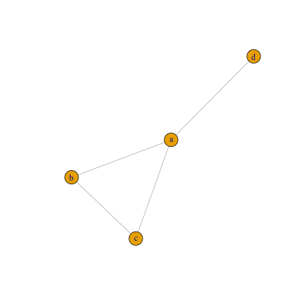<!-- --> ] <style> .panel1-igraph1-rotate { color: black; width: 38.6060606060606%; hight: 32%; float: left; padding-left: 1%; font-size: 80% } .panel2-igraph1-rotate { color: black; width: 59.3939393939394%; hight: 32%; float: left; padding-left: 1%; font-size: 80% } .panel3-igraph1-rotate { color: black; width: NA%; hight: 33%; float: left; padding-left: 1%; font-size: 80% } </style> --- count: false ### Create a simple directed graph .panel1-igraph1b-rotate[ ```r g2 <- igraph::graph_from_literal(a+-+b, b--+c, c--+a, a+-+d) *g2 ``` ] .panel2-igraph1b-rotate[ ``` IGRAPH f82780b DN-- 4 6 -- + attr: name (v/c) + edges from f82780b (vertex names): [1] a->b a->d b->a b->c c->a d->a ``` ] --- count: false ### Create a simple directed graph .panel1-igraph1b-rotate[ ```r g2 <- igraph::graph_from_literal(a+-+b, b--+c, c--+a, a+-+d) *V(g2) ``` ] .panel2-igraph1b-rotate[ ``` + 4/4 vertices, named, from c10494a: [1] a b c d ``` ] --- count: false ### Create a simple directed graph .panel1-igraph1b-rotate[ ```r g2 <- igraph::graph_from_literal(a+-+b, b--+c, c--+a, a+-+d) *E(g2) ``` ] .panel2-igraph1b-rotate[ ``` + 6/6 edges from 975cee4 (vertex names): [1] a->b a->d b->a b->c c->a d->a ``` ] --- count: false ### Create a simple directed graph .panel1-igraph1b-rotate[ ```r g2 <- igraph::graph_from_literal(a+-+b, b--+c, c--+a, a+-+d) *plot(g2) ``` ] .panel2-igraph1b-rotate[ 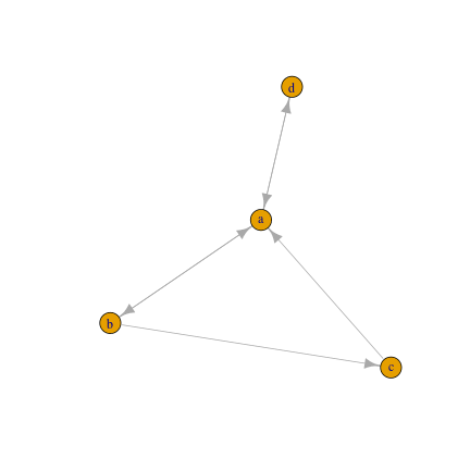<!-- --> ] <style> .panel1-igraph1b-rotate { color: black; width: 38.6060606060606%; hight: 32%; float: left; padding-left: 1%; font-size: 80% } .panel2-igraph1b-rotate { color: black; width: 59.3939393939394%; hight: 32%; float: left; padding-left: 1%; font-size: 80% } .panel3-igraph1b-rotate { color: black; width: NA%; hight: 33%; float: left; padding-left: 1%; font-size: 80% } </style> --- layout:true ## Visualization (igraph) --- count: false ### Create a graph from adjacency matrix .panel1-igraph2am-rotate[ ```r am <- matrix(c(0, 1, 1, 1, 1, 0, 1, 0, 1, 1, 0, 0, 1, 0, 0, 0), nrow=4,ncol=4,byrow=TRUE) rownames(am) <- c('a','b','c','d') colnames(am) <- c('a','b','c','d') gu <- graph_from_adjacency_matrix(am) *knitr::kable(am) ``` ] .panel2-igraph2am-rotate[ <table> <thead> <tr> <th style="text-align:left;"> </th> <th style="text-align:right;"> a </th> <th style="text-align:right;"> b </th> <th style="text-align:right;"> c </th> <th style="text-align:right;"> d </th> </tr> </thead> <tbody> <tr> <td style="text-align:left;"> a </td> <td style="text-align:right;"> 0 </td> <td style="text-align:right;"> 1 </td> <td style="text-align:right;"> 1 </td> <td style="text-align:right;"> 1 </td> </tr> <tr> <td style="text-align:left;"> b </td> <td style="text-align:right;"> 1 </td> <td style="text-align:right;"> 0 </td> <td style="text-align:right;"> 1 </td> <td style="text-align:right;"> 0 </td> </tr> <tr> <td style="text-align:left;"> c </td> <td style="text-align:right;"> 1 </td> <td style="text-align:right;"> 1 </td> <td style="text-align:right;"> 0 </td> <td style="text-align:right;"> 0 </td> </tr> <tr> <td style="text-align:left;"> d </td> <td style="text-align:right;"> 1 </td> <td style="text-align:right;"> 0 </td> <td style="text-align:right;"> 0 </td> <td style="text-align:right;"> 0 </td> </tr> </tbody> </table> ] --- count: false ### Create a graph from adjacency matrix .panel1-igraph2am-rotate[ ```r am <- matrix(c(0, 1, 1, 1, 1, 0, 1, 0, 1, 1, 0, 0, 1, 0, 0, 0), nrow=4,ncol=4,byrow=TRUE) rownames(am) <- c('a','b','c','d') colnames(am) <- c('a','b','c','d') gu <- graph_from_adjacency_matrix(am) *gu ``` ] .panel2-igraph2am-rotate[ ``` IGRAPH 251c4dc DN-- 4 8 -- + attr: name (v/c) + edges from 251c4dc (vertex names): [1] a->b a->c a->d b->a b->c c->a c->b d->a ``` ] --- count: false ### Create a graph from adjacency matrix .panel1-igraph2am-rotate[ ```r am <- matrix(c(0, 1, 1, 1, 1, 0, 1, 0, 1, 1, 0, 0, 1, 0, 0, 0), nrow=4,ncol=4,byrow=TRUE) rownames(am) <- c('a','b','c','d') colnames(am) <- c('a','b','c','d') gu <- graph_from_adjacency_matrix(am) *plot(gu) ``` ] .panel2-igraph2am-rotate[ 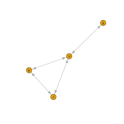<!-- --> ] <style> .panel1-igraph2am-rotate { color: black; width: 38.6060606060606%; hight: 32%; float: left; padding-left: 1%; font-size: 80% } .panel2-igraph2am-rotate { color: black; width: 59.3939393939394%; hight: 32%; float: left; padding-left: 1%; font-size: 80% } .panel3-igraph2am-rotate { color: black; width: NA%; hight: 33%; float: left; padding-left: 1%; font-size: 80% } </style> --- count: false ### Create a graph from edgelist .panel1-igraph2el-rotate[ ```r el <- data.frame("from"=c('a','b','c','a'), "to"=c('b','c','a','d')) g3 <- graph_from_data_frame(el,directed = FALSE) *g3 ``` ] .panel2-igraph2el-rotate[ ``` IGRAPH ed415c7 UN-- 4 4 -- + attr: name (v/c) + edges from ed415c7 (vertex names): [1] a--b b--c a--c a--d ``` ] --- count: false ### Create a graph from edgelist .panel1-igraph2el-rotate[ ```r el <- data.frame("from"=c('a','b','c','a'), "to"=c('b','c','a','d')) g3 <- graph_from_data_frame(el,directed = FALSE) *plot(g3) ``` ] .panel2-igraph2el-rotate[ 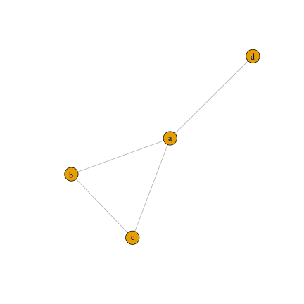<!-- --> ] <style> .panel1-igraph2el-rotate { color: black; width: 38.6060606060606%; hight: 32%; float: left; padding-left: 1%; font-size: 80% } .panel2-igraph2el-rotate { color: black; width: 59.3939393939394%; hight: 32%; float: left; padding-left: 1%; font-size: 80% } .panel3-igraph2el-rotate { color: black; width: NA%; hight: 33%; float: left; padding-left: 1%; font-size: 80% } </style> --- count: false ### Weighted directed graph .panel1-igraphwdir-rotate[ ```r amd <- matrix(c(0, 0.5, 0, 3, 8, 0, 1, 0, 1, 0, 0, 0, 2, 0, 0, 0), nrow=4,ncol=4,byrow=TRUE) rownames(amd) <- c('a','b','c','d') colnames(amd) <- c('a','b','c','d') gwd <- igraph::graph_from_adjacency_matrix(amd, weighted = TRUE, mode = 'directed') l <- layout.reingold.tilford(gwd) *knitr::kable(amd) ``` ] .panel2-igraphwdir-rotate[ <table> <thead> <tr> <th style="text-align:left;"> </th> <th style="text-align:right;"> a </th> <th style="text-align:right;"> b </th> <th style="text-align:right;"> c </th> <th style="text-align:right;"> d </th> </tr> </thead> <tbody> <tr> <td style="text-align:left;"> a </td> <td style="text-align:right;"> 0 </td> <td style="text-align:right;"> 0.5 </td> <td style="text-align:right;"> 0 </td> <td style="text-align:right;"> 3 </td> </tr> <tr> <td style="text-align:left;"> b </td> <td style="text-align:right;"> 8 </td> <td style="text-align:right;"> 0.0 </td> <td style="text-align:right;"> 1 </td> <td style="text-align:right;"> 0 </td> </tr> <tr> <td style="text-align:left;"> c </td> <td style="text-align:right;"> 1 </td> <td style="text-align:right;"> 0.0 </td> <td style="text-align:right;"> 0 </td> <td style="text-align:right;"> 0 </td> </tr> <tr> <td style="text-align:left;"> d </td> <td style="text-align:right;"> 2 </td> <td style="text-align:right;"> 0.0 </td> <td style="text-align:right;"> 0 </td> <td style="text-align:right;"> 0 </td> </tr> </tbody> </table> ] --- count: false ### Weighted directed graph .panel1-igraphwdir-rotate[ ```r amd <- matrix(c(0, 0.5, 0, 3, 8, 0, 1, 0, 1, 0, 0, 0, 2, 0, 0, 0), nrow=4,ncol=4,byrow=TRUE) rownames(amd) <- c('a','b','c','d') colnames(amd) <- c('a','b','c','d') gwd <- igraph::graph_from_adjacency_matrix(amd, weighted = TRUE, mode = 'directed') l <- layout.reingold.tilford(gwd) *gwd ``` ] .panel2-igraphwdir-rotate[ ``` IGRAPH 496e01f DNW- 4 6 -- + attr: name (v/c), weight (e/n) + edges from 496e01f (vertex names): [1] a->b a->d b->a b->c c->a d->a ``` ] --- count: false ### Weighted directed graph .panel1-igraphwdir-rotate[ ```r amd <- matrix(c(0, 0.5, 0, 3, 8, 0, 1, 0, 1, 0, 0, 0, 2, 0, 0, 0), nrow=4,ncol=4,byrow=TRUE) rownames(amd) <- c('a','b','c','d') colnames(amd) <- c('a','b','c','d') gwd <- igraph::graph_from_adjacency_matrix(amd, weighted = TRUE, mode = 'directed') l <- layout.reingold.tilford(gwd) *E(gwd)$weight ``` ] .panel2-igraphwdir-rotate[ ``` [1] 0.5 3.0 8.0 1.0 1.0 2.0 ``` ] --- count: false ### Weighted directed graph .panel1-igraphwdir-rotate[ ```r amd <- matrix(c(0, 0.5, 0, 3, 8, 0, 1, 0, 1, 0, 0, 0, 2, 0, 0, 0), nrow=4,ncol=4,byrow=TRUE) rownames(amd) <- c('a','b','c','d') colnames(amd) <- c('a','b','c','d') gwd <- igraph::graph_from_adjacency_matrix(amd, weighted = TRUE, mode = 'directed') l <- layout.reingold.tilford(gwd) *plot(gwd,layout=l) ``` ] .panel2-igraphwdir-rotate[ 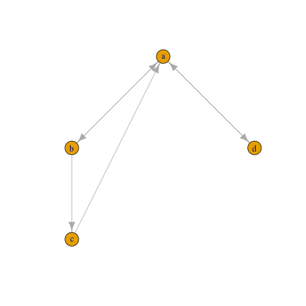<!-- --> ] --- count: false ### Weighted directed graph .panel1-igraphwdir-rotate[ ```r amd <- matrix(c(0, 0.5, 0, 3, 8, 0, 1, 0, 1, 0, 0, 0, 2, 0, 0, 0), nrow=4,ncol=4,byrow=TRUE) rownames(amd) <- c('a','b','c','d') colnames(amd) <- c('a','b','c','d') gwd <- igraph::graph_from_adjacency_matrix(amd, weighted = TRUE, mode = 'directed') l <- layout.reingold.tilford(gwd) *plot(gwd,edge.width=E(gwd)$weight,layout=l) ``` ] .panel2-igraphwdir-rotate[ 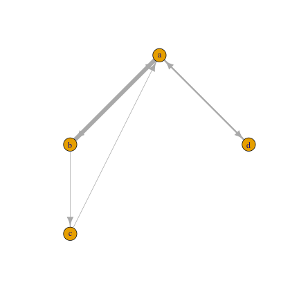<!-- --> ] <style> .panel1-igraphwdir-rotate { color: black; width: 38.6060606060606%; hight: 32%; float: left; padding-left: 1%; font-size: 80% } .panel2-igraphwdir-rotate { color: black; width: 59.3939393939394%; hight: 32%; float: left; padding-left: 1%; font-size: 80% } .panel3-igraphwdir-rotate { color: black; width: NA%; hight: 33%; float: left; padding-left: 1%; font-size: 80% } </style> --- count: false ### Plotting layouts with igraph .panel1-igraphrand1-rotate[ ```r set.seed(1234) gr <- sample_grg(100, 0.2) *ll <- igraph::layout.circle(gr) plot(gr,layout=ll) ``` ] .panel2-igraphrand1-rotate[ 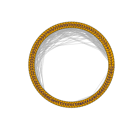<!-- --> ] --- count: false ### Plotting layouts with igraph .panel1-igraphrand1-rotate[ ```r set.seed(1234) gr <- sample_grg(100, 0.2) *ll <- igraph::layout.kamada.kawai(gr) plot(gr,layout=ll) ``` ] .panel2-igraphrand1-rotate[ 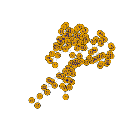<!-- --> ] --- count: false ### Plotting layouts with igraph .panel1-igraphrand1-rotate[ ```r set.seed(1234) gr <- sample_grg(100, 0.2) *ll <- igraph::layout.random(gr) plot(gr,layout=ll) ``` ] .panel2-igraphrand1-rotate[ <!-- --> ] --- count: false ### Plotting layouts with igraph .panel1-igraphrand1-rotate[ ```r set.seed(1234) gr <- sample_grg(100, 0.2) *ll <- layout.fruchterman.reingold(gr) plot(gr,layout=ll) ``` ] .panel2-igraphrand1-rotate[ <!-- --> ] <style> .panel1-igraphrand1-rotate { color: black; width: 38.6060606060606%; hight: 32%; float: left; padding-left: 1%; font-size: 80% } .panel2-igraphrand1-rotate { color: black; width: 59.3939393939394%; hight: 32%; float: left; padding-left: 1%; font-size: 80% } .panel3-igraphrand1-rotate { color: black; width: NA%; hight: 33%; float: left; padding-left: 1%; font-size: 80% } </style> --- count: false ### Plotting layouts with ggraph .panel1-ggraph-rotate[ ```r library(ggraph) *ggl <- 'gem' ggraph(gr, layout=ggl) + geom_edge_link(colour="lightblue") + geom_node_point(size=3) + theme_graph() ``` ] .panel2-ggraph-rotate[ <!-- --> ] --- count: false ### Plotting layouts with ggraph .panel1-ggraph-rotate[ ```r library(ggraph) *ggl <- 'kk' ggraph(gr, layout=ggl) + geom_edge_link(colour="lightblue") + geom_node_point(size=3) + theme_graph() ``` ] .panel2-ggraph-rotate[ <!-- --> ] --- count: false ### Plotting layouts with ggraph .panel1-ggraph-rotate[ ```r library(ggraph) *ggl <- 'drl' ggraph(gr, layout=ggl) + geom_edge_link(colour="lightblue") + geom_node_point(size=3) + theme_graph() ``` ] .panel2-ggraph-rotate[ 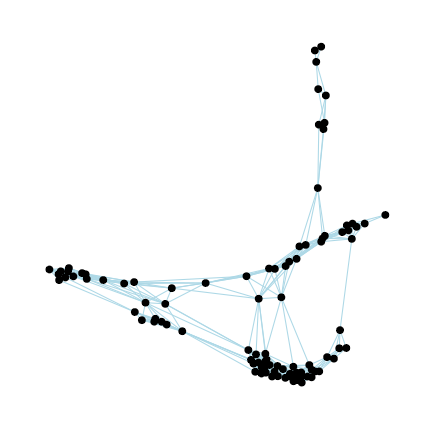<!-- --> ] --- count: false ### Plotting layouts with ggraph .panel1-ggraph-rotate[ ```r library(ggraph) *ggl <- 'graphopt' ggraph(gr, layout=ggl) + geom_edge_link(colour="lightblue") + geom_node_point(size=3) + theme_graph() ``` ] .panel2-ggraph-rotate[ 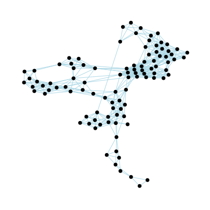<!-- --> ] <style> .panel1-ggraph-rotate { color: black; width: 38.6060606060606%; hight: 32%; float: left; padding-left: 1%; font-size: 80% } .panel2-ggraph-rotate { color: black; width: 59.3939393939394%; hight: 32%; float: left; padding-left: 1%; font-size: 80% } .panel3-ggraph-rotate { color: black; width: NA%; hight: 33%; float: left; padding-left: 1%; font-size: 80% } </style> --- layout:true ## Network indices (igraph) --- count: false ### Some indices .panel1-igraphindices-user[ ```r *nodesel <- 2 # Centrality measures *degr <- centr_degree(gr) # Degree *betw <- centr_betw(gr) # Betweenness *clos <- centr_clo(gr) # Closeness *prk <- igraph::page.rank(gr)$vector # Pagerank ``` ] .panel2-igraphindices-user[ ] --- count: false ### Some indices .panel1-igraphindices-user[ ```r nodesel <- 2 # Centrality measures degr <- centr_degree(gr) # Degree betw <- centr_betw(gr) # Betweenness clos <- centr_clo(gr) # Closeness prk <- igraph::page.rank(gr)$vector # Pagerank *cat("Centrality measures of node",nodesel,":\n\n", * " degree: ",degr$res[nodesel],"\n", * " betweenness: ",betw$res[nodesel],"\n", * " closeness: ",clos$res[nodesel],"\n", * " pagerank: ",prk[nodesel],"\n") ``` ] .panel2-igraphindices-user[ ``` Centrality measures of node 2 : degree: 9 betweenness: 2.994037 closeness: 0.2605263 pagerank: 0.006933141 ``` ] --- count: false ### Some indices .panel1-igraphindices-user[ ```r nodesel <- 2 # Centrality measures degr <- centr_degree(gr) # Degree betw <- centr_betw(gr) # Betweenness clos <- centr_clo(gr) # Closeness prk <- igraph::page.rank(gr)$vector # Pagerank cat("Centrality measures of node",nodesel,":\n\n", " degree: ",degr$res[nodesel],"\n", " betweenness: ",betw$res[nodesel],"\n", " closeness: ",clos$res[nodesel],"\n", " pagerank: ",prk[nodesel],"\n") # Network Centralization *cat("Network centralization:\n\n", * " degree: ",degr$centralization,"\n", * " betweenness: ",betw$centralization,"\n", * " closeness: ",clos$centralization,"\n") ``` ] .panel2-igraphindices-user[ ``` Centrality measures of node 2 : degree: 9 betweenness: 2.994037 closeness: 0.2605263 pagerank: 0.006933141 ``` ``` Network centralization: degree: 0.1244444 betweenness: 0.1212017 closeness: 0.1796426 ``` ] --- count: false ### Some indices .panel1-igraphindices-user[ ```r nodesel <- 2 # Centrality measures degr <- centr_degree(gr) # Degree betw <- centr_betw(gr) # Betweenness clos <- centr_clo(gr) # Closeness prk <- igraph::page.rank(gr)$vector # Pagerank cat("Centrality measures of node",nodesel,":\n\n", " degree: ",degr$res[nodesel],"\n", " betweenness: ",betw$res[nodesel],"\n", " closeness: ",clos$res[nodesel],"\n", " pagerank: ",prk[nodesel],"\n") # Network Centralization cat("Network centralization:\n\n", " degree: ",degr$centralization,"\n", " betweenness: ",betw$centralization,"\n", " closeness: ",clos$centralization,"\n") # Network diameter *cat("Network diameter:",diameter(gr)) ``` ] .panel2-igraphindices-user[ ``` Centrality measures of node 2 : degree: 9 betweenness: 2.994037 closeness: 0.2605263 pagerank: 0.006933141 ``` ``` Network centralization: degree: 0.1244444 betweenness: 0.1212017 closeness: 0.1796426 ``` ``` Network diameter: 11 ``` ] --- count: false ### Some indices .panel1-igraphindices-user[ ```r nodesel <- 2 # Centrality measures degr <- centr_degree(gr) # Degree betw <- centr_betw(gr) # Betweenness clos <- centr_clo(gr) # Closeness prk <- igraph::page.rank(gr)$vector # Pagerank cat("Centrality measures of node",nodesel,":\n\n", " degree: ",degr$res[nodesel],"\n", " betweenness: ",betw$res[nodesel],"\n", " closeness: ",clos$res[nodesel],"\n", " pagerank: ",prk[nodesel],"\n") # Network Centralization cat("Network centralization:\n\n", " degree: ",degr$centralization,"\n", " betweenness: ",betw$centralization,"\n", " closeness: ",clos$centralization,"\n") # Network diameter cat("Network diameter:",diameter(gr)) *# Triad census (directed graphs) # Triad census (directed graphs) *cat("Triad census: \n") *triad.census(gwd) ``` ] .panel2-igraphindices-user[ ``` Centrality measures of node 2 : degree: 9 betweenness: 2.994037 closeness: 0.2605263 pagerank: 0.006933141 ``` ``` Network centralization: degree: 0.1244444 betweenness: 0.1212017 closeness: 0.1796426 ``` ``` Network diameter: 11 ``` ``` Triad census: ``` ``` [1] 0 1 0 0 0 0 1 0 0 0 1 0 0 1 0 0 ``` ] --- count: false ### Some indices .panel1-igraphindices-user[ ```r nodesel <- 2 # Centrality measures degr <- centr_degree(gr) # Degree betw <- centr_betw(gr) # Betweenness clos <- centr_clo(gr) # Closeness prk <- igraph::page.rank(gr)$vector # Pagerank cat("Centrality measures of node",nodesel,":\n\n", " degree: ",degr$res[nodesel],"\n", " betweenness: ",betw$res[nodesel],"\n", " closeness: ",clos$res[nodesel],"\n", " pagerank: ",prk[nodesel],"\n") # Network Centralization cat("Network centralization:\n\n", " degree: ",degr$centralization,"\n", " betweenness: ",betw$centralization,"\n", " closeness: ",clos$centralization,"\n") # Network diameter cat("Network diameter:",diameter(gr)) # Triad census (directed graphs) # Triad census (directed graphs) cat("Triad census: \n") triad.census(gwd) ``` ] .panel2-igraphindices-user[ ``` Centrality measures of node 2 : degree: 9 betweenness: 2.994037 closeness: 0.2605263 pagerank: 0.006933141 ``` ``` Network centralization: degree: 0.1244444 betweenness: 0.1212017 closeness: 0.1796426 ``` ``` Network diameter: 11 ``` ``` Triad census: ``` ``` [1] 0 1 0 0 0 0 1 0 0 0 1 0 0 1 0 0 ``` ] <style> .panel1-igraphindices-user { color: black; width: 38.6060606060606%; hight: 32%; float: left; padding-left: 1%; font-size: 80% } .panel2-igraphindices-user { color: black; width: 59.3939393939394%; hight: 32%; float: left; padding-left: 1%; font-size: 80% } .panel3-igraphindices-user { color: black; width: NA%; hight: 33%; float: left; padding-left: 1%; font-size: 80% } </style> --- layout:false class: inverse, middle, center # 2. Networks and Football --- layout:true # Networks and Football? --- When comes to defining a network, it is crucial to define the agents and the mechanics that determine the generation of relationships between them. Since football (as well as other team sports) is a game involving different level of complexity, different perspective can be taken into account, we start from three concepts: .center[ **the topic**: relationships between football players and/or teams **the context**: interactions of players on the pitch, player transfers during a market session **the application**: evaluate player performances, predict match results, analyse player transfers ] --- .pull-left[ ## Passing network <img src="img/prova_grafo_Napoli.png" width="80%" style="display: block; margin: auto;" /> ] .pull-right[ ## Transfer market network <img src="img/Traditore.png" width="90%" style="display: block; margin: auto;" /> ] --- class: left .pull-left[ ## Passing network - directed network - weighted network - network bounds are clearly defined - low number of nodes - network is highly connected - node attributes: role, player skills, ... - edge attributes: nr. passes, nr. long passes, ... ] .pull-right[ ## Transfer market network - directed network - weighted network - network bounds are not easy to define - high number of nodes - network is highly connected - node attributes: team features - edge attributes: market value, player agent, ... ] --- layout:false ## Data description #### Passing Network 1. Group Stage matches of UEFA Champions League among three consecutive seasons. + from 2016-2017 to 2018-2019 + 288 matches and 576 passing networks 2. Group Stage matches of UEFA Champions League. + 2016-2017 season + 32-teams, 96 matches and 192 passing networks #### Transfer market network 3. 2019 Italian Serie A transfer market. + Italian football transfer market session of season 2019-2020 + Focus on the 20 Italian Serie A teams --- ### Example of an adjacency matrix in football Team passing network of Arsenal (Arsenal vs. PSG, 09/13/2016), Group Stage match of the 2016-2017 UCL | | | `\(p_1\)` | `\(p_2\)` | `\(p_3\)` | `\(p_4\)` | `\(p_5\)` | `\(p_6\)` | `\(p_7\)` | `\(p_8\)` | `\(p_9\)` | `\(p_{10}\)` | `\(p_{11}\)` | |---|---|:---:|:---:|:---:|:---:|:---:|:---:|:---:|:---:|:---:|:---:|:---:| | Ospina | `\(p_{1}\)` | | 1 | 1 | 1 | 1 | 1 | 4 | 1 | 11 | 2 | 1 | | Koscielny | `\(p_{2}\)` | 1 | | 3 | 2 | 0 | 1 | 13 | 11 | 12 | 1 | 1 | | Alexis Sanchez | `\(p_{3}\)` | 0 | 3 | | 9 | 4 | 4 | 0 | 4 | 0 | 2 | 4 | | Ozil | `\(p_{4}\)` | 0 | 2 | 8 | | 2 | 8 | 3 | 6 | 2 | 3 | 5 | | Oxlade-Chamberlain | `\(p_{5}\)` | 0 | 2 | 2 | 2 | | 0 | 0 | 4 | 0 | 2 | 1 | | Iwobi | `\(p_{6}\)` | 0 | 4 | 6 | 8 | 0 | | 7 | 3 | 4 | 4 | 2 | | Monreal | `\(p_{7}\)` | 3 | 3 | 8 | 2 | 3 | 7 | | 5 | 1 | 0 | 6 | | Santi Cazorla | `\(p_{8}\)` | 0 | 10 | 11 | 13 | 5 | 7 | 5 | | 8 | 7 | 6 | | Mustafi | `\(p_{9}\)` | 6 | 13 | 1 | 1 | 2 | 2 | 0 | 15 | | 13 | 1 | | Bellerin | `\(p_{10}\)` | 1 | 0 | 2 | 1 | 4 | 5 | 0 | 2 | 11 | | 3 | | Coquelin | `\(p_{11}\)` | 0 | 3 | 5 | 3 | 1 | 4 | 3 | 9 | 2 | 3 | --- ### The passing network visualized <img src="img/grafofull_sez2.jpg" width="2337" height="550px" style="display: block; margin: auto;" /> --- <img src="img/Arsenallineup_mod.png" width="1116" height="550px" style="display: block; margin: auto;" /> <!-- fonte: pagina "archivio" sezione UCL diretta.it --> --- ### A simplified visualization .center[.content-box-blue[ Objective: emphasize most influential relationships in terms of passes. ]] Let us consider two representative matches (Group Stage, 2016-2017 UCL): 1) **Barcelona:** Barcelona vs. Borussia 'Gladbach (4-0), 06/12/2016 + 939 completed passes, with approximately `\(92\%\)` accuracy + maximum number of completed passes in the data 2) **Rostov:** Rostov vs. Bayern Munchen (3-2), 11/23/2016 + 297 completed passes, high ball possession + maximum number of completed passes in the data .center[.content-box-blue[ Visual representation: normalize the weights with respect to all the passes that occurred among players during the entire match and emphasize the most influential ties (solid line) ]] --- ### Barcelona: Tiki-taka <img src="img/barca1.png" width="828" height="550px" style="display: block; margin: auto;" /> --- ### Team lineup: Barcelona <img src="img/barcalineup.png" width="1117" height="550px" style="display: block; margin: auto;" /> --- ### Rostov: a defensive strategy <img src="img/rostov1.png" width="697" height="550px" style="display: block; margin: auto;" /> --- ### Team lineup: Rostov <img src="img/rostovlineup.png" width="1112" height="550px" style="display: block; margin: auto;" /> --- ## Summarising... .pull-left[ - most relevant arcs are represented by **solid lines** - **dashed lines** represent less important links - emphasize importance of players in a network is in terms of **out-degree centrality** ] .pull-right[ - set the size of all vertices depending on the number of completed passes (which players are more involved in cooperation processes?) ] - Barcelona shows the well-known "tiki-taka" style of play: ball possession and numerous short passes + 5 large-sized players, including the three midfielders + key role of central defenders in starting the offensive actions + strong relationship between Lionel Messi, Iniesta and Denis Suarez + right-wing Arda Turan mostly cooperates with his right back Lucas Digne - Rostov's passing network suggests a more defensive strategy + the goalkeeper plays a central role in ball possession, tending to pass directly to the right midfielders + the outdegrees of central forwards are comparable with respect to the other players + the central midfielder Alexandru Gatskan could be considered the lighthouse of Rostov + central defenders seem to have a less important role in possessing the ball, especially compared Barcelona's previous counterparts (Mascherano and Umtiti) --- class: inverse, middle, center # 3. Passing Network ## Identify styles of play --- # Triad census > A team of experts is not necessarily an expert team. > > Clemente (2016) - Use triad census to unveil "hidden" aspects regarding cohesion between players and their roles on the pitch. There are **16 equivalence classes** associated with triadic relationships between three distinct nodes: <img src="img/triads_base.png" width="100%" style="display: block; margin: auto;" /> --- <embed src="img/boxplot_spaghetti.pdf" width="100%" height="90%" style="display: block; margin: auto;" type="application/pdf" /> --- # Deviations from random scenario The empirical distribution of raw triad census is able to characterize the network structure and can help to understand specific features of this framework. In addition triad census can help to identify different styles of play. -- > Question: > > Is it possible to "measure" the possible deviation against a random network structure in the data? -- - `\(\tau_{i}\)` scores: $$ \tau_{i} = \dfrac{T_i- E(T_i)}{\sqrt{Var(T_i)}}, $$ for each isomorphism class `\(T_i\)`, with `\(i = 1, \ldots, 16\)`. Scores represent the standardized departures of observed triads from the theoretical random distribution. -- .center[.content-box-blue[ `\(\tau_{i}\)` can be useful to asses whether the observed triadic distribution deviates from randomness. ]] --- <embed src="img/boxplot_triadi_peranno.pdf" width="100%" height="90%" style="display: block; margin: auto;" type="application/pdf" /> --- <embed src="img/triadi_top10.pdf" width="100%" height="90%" style="display: block; margin: auto;" type="application/pdf" /> --- # Identify styles of play 1. Apply Correspondence Analysis on triad census. 2. Apply k-means clustering to establish a set of styles of play This allows us to identify a set of triadic profiles which are related to different triadic behaviour in football. Four resulting centroids are the identified: * **T1**, presents a number of `102` and `201` greater than the general medians. * **T2**, presents lower `201` and greater `210` and `120` (D,U,C) types. * **T3**, shows the highest counts of full connected triads, i.e. `300` (exceeding the general median of 22 units). * **T4**, exhibits the lower value of this class and the higher counts of triads with low number of links, i.e. `012` and `102`. --- # Summarising... - Triad census is capable to unveil hidden features involving teams, matches and competitions - It is possible to characterize styles of play combining Network Analysis and statistical models .blue[**Further Developments**] - use of more sophisticated unsupervised ML models - rank (European) teams w.r.t. different styles of play - statistical testing for deviations from a prefixed scenario --- class: inverse, middle, center # 3. Passing Network ## Predicting match outcomes --- layout: true # Performance Indicators Derived from Passing Networks --- Topological properties of the network can help to identify relevant structures and hidden features underlying passes in football (or even in other team sports), and can be profitably used to obtain performance measures at the team and the player level. -- .center[.content-box-blue[ Focus on a restricted number of indices able to capture the complexity of the network topology and have a meaningful interpretation for football and other team sports. ]] -- Network summary measures can be divided into three main categories: *Macro indices* describe the overall characteristics of a network, while *micro indices* focus on the individual nodes. Measures that combine information from the micro- and macro-levels are usually denoted as *meso-level* measures. --- layout: true # Macro-level indices in football --- > - **Total number of passes** > > It is a simple team-level summary indices, i.e. the number of links occurring in the network, corresponding to the absolute number of total passes conducted between teammates during the match. A higher value of this index reveals strong cooperation between team players, who successfully interact with each other. --- count: false <table> <caption>Total completed passes by a team in each match, 2016--2017 UCL (Group Stage).</caption> <thead> <tr> <th style="text-align:left;"> Team </th> <th style="text-align:left;"> I </th> <th style="text-align:left;"> II </th> <th style="text-align:left;"> III </th> <th style="text-align:left;"> IV </th> <th style="text-align:left;"> V </th> <th style="text-align:left;"> VI </th> <th style="text-align:left;"> Total </th> </tr> </thead> <tbody> <tr> <td style="text-align:left;"> 1 Bayern München </td> <td style="text-align:left;"> 721 </td> <td style="text-align:left;"> 612 </td> <td style="text-align:left;"> 787 </td> <td style="text-align:left;"> 728 </td> <td style="text-align:left;"> 645 </td> <td style="text-align:left;"> 759 </td> <td style="text-align:left;"> 4252 </td> </tr> <tr> <td style="text-align:left;"> 2 Barcelona </td> <td style="text-align:left;"> 772 </td> <td style="text-align:left;"> 615 </td> <td style="text-align:left;"> 383 </td> <td style="text-align:left;"> 521 </td> <td style="text-align:left;"> 649 </td> <td style="text-align:left;"> 939 </td> <td style="text-align:left;"> 3879 </td> </tr> <tr> <td style="text-align:left;"> 3 PSG </td> <td style="text-align:left;"> 519 </td> <td style="text-align:left;"> 725 </td> <td style="text-align:left;"> 647 </td> <td style="text-align:left;"> 658 </td> <td style="text-align:left;"> 557 </td> <td style="text-align:left;"> 534 </td> <td style="text-align:left;"> 3640 </td> </tr> <tr> <td style="text-align:left;"> 4 Borussia Dortmund </td> <td style="text-align:left;"> 580 </td> <td style="text-align:left;"> 603 </td> <td style="text-align:left;"> 451 </td> <td style="text-align:left;"> 519 </td> <td style="text-align:left;"> 737 </td> <td style="text-align:left;"> 533 </td> <td style="text-align:left;"> 3423 </td> </tr> <tr> <td style="text-align:left;"> 5 Juventus </td> <td style="text-align:left;"> 448 </td> <td style="text-align:left;"> 744 </td> <td style="text-align:left;"> 492 </td> <td style="text-align:left;"> 515 </td> <td style="text-align:left;"> 467 </td> <td style="text-align:left;"> 618 </td> <td style="text-align:left;"> 3284 </td> </tr> </tbody> </table> --- count: false <table> <caption>Total completed passes by a team in each match, 2016--2017 UCL (Group Stage).</caption> <thead> <tr> <th style="text-align:left;"> </th> <th style="text-align:left;"> Team </th> <th style="text-align:left;"> I </th> <th style="text-align:left;"> II </th> <th style="text-align:left;"> III </th> <th style="text-align:left;"> IV </th> <th style="text-align:left;"> V </th> <th style="text-align:left;"> VI </th> <th style="text-align:left;"> Total </th> </tr> </thead> <tbody> <tr> <td style="text-align:left;"> 7 </td> <td style="text-align:left;"> 28 Legia Warsav </td> <td style="text-align:left;"> 221 </td> <td style="text-align:left;"> 336 </td> <td style="text-align:left;"> 349 </td> <td style="text-align:left;"> 452 </td> <td style="text-align:left;"> 254 </td> <td style="text-align:left;"> 278 </td> <td style="text-align:left;"> 1890 </td> </tr> <tr> <td style="text-align:left;"> 8 </td> <td style="text-align:left;"> 29 CSKA Moskov </td> <td style="text-align:left;"> 244 </td> <td style="text-align:left;"> 237 </td> <td style="text-align:left;"> 295 </td> <td style="text-align:left;"> 314 </td> <td style="text-align:left;"> 388 </td> <td style="text-align:left;"> 218 </td> <td style="text-align:left;"> 1696 </td> </tr> <tr> <td style="text-align:left;"> 9 </td> <td style="text-align:left;"> 30 Leicester </td> <td style="text-align:left;"> 275 </td> <td style="text-align:left;"> 223 </td> <td style="text-align:left;"> 277 </td> <td style="text-align:left;"> 306 </td> <td style="text-align:left;"> 370 </td> <td style="text-align:left;"> 213 </td> <td style="text-align:left;"> 1664 </td> </tr> <tr> <td style="text-align:left;"> 10 </td> <td style="text-align:left;"> 31 Dynamo Zagreb </td> <td style="text-align:left;"> 341 </td> <td style="text-align:left;"> 246 </td> <td style="text-align:left;"> 167 </td> <td style="text-align:left;"> 203 </td> <td style="text-align:left;"> 285 </td> <td style="text-align:left;"> 328 </td> <td style="text-align:left;"> 1570 </td> </tr> <tr> <td style="text-align:left;"> 11 </td> <td style="text-align:left;"> 32 Rostov </td> <td style="text-align:left;"> 179 </td> <td style="text-align:left;"> 370 </td> <td style="text-align:left;"> 213 </td> <td style="text-align:left;"> 197 </td> <td style="text-align:left;"> 130 </td> <td style="text-align:left;"> 223 </td> <td style="text-align:left;"> 1312 </td> </tr> </tbody> </table> <style> .panel1-tab_CLtotpass-rotate { color: black; width: 99%; hight: 32%; float: left; padding-left: 1%; font-size: 80% } .panel2-tab_CLtotpass-rotate { color: black; width: NA%; hight: 32%; float: left; padding-left: 1%; font-size: 80% } .panel3-tab_CLtotpass-rotate { color: black; width: NA%; hight: 33%; float: left; padding-left: 1%; font-size: 80% } </style> --- > - **Network diameter** > > This measure is expressed as the *geodesic* distance between the most distant nodes of a graph, representing the extent of the graph and the topological length between the two most distant nodes, without taking into account the link weights. A team with a high network diameter reflects the team's ability to generate as many direct connections as possible, even in terms of passes. --- > - **Reciprocity** > > This index is computed as the proportion of mutual connections in a directed graph, i.e., the probability that the opposite counterpart of a directed edge is included in the graph. Reciprocity measures the ability of two players to have mutual connections. A team expressing many null or reciprocated ties may be different from one that has asymmetric connections (which might be a hierarchy). --- > - **Assortativity** > > Assortativity coefficient measures the level of homophily for a graph; this coefficient, based on the degree of vertices, is normalized and takes values in the interval `\([-1,1]\)`. High assortativity means that players who have an equal or similar number of passes are often connected. Otherwise, low-degree players are more likely be connected to teammates with a high degree of passing. --- layout: true # Micro-level indices in football --- > - **Cliques** > > Several individual indices involve subgroups of players considering complete subgraphs within a network, also denoted as *cliques*. Cliques can be helpful to understand the structure of interactions between teammates and the regularity of such connections. Two useful indices can be computed: the size of the *largest clique*, representing the number of vertices which contains the largest clique, and the number of many times the *maximal clique* occurs, denoted as the *countmax cliques*. In this case, it is possible to identify the size and regularity of the denser passing structures occurring in a match. However, when measuring cliques, directional properties may be lost. --- > - **Clustering coefficient** > > The generalized *clustering coefficient*, based on the transitivity property, is a measure used to detect the fraction of closest triplets in directed networks. The coefficient is also a normalized index and takes a value within the interval `\([0,1]\)`. When the value is closer to one, the passing triplets between teammates are dense. This index can be used to identify patterns of interactions between teammates based on their so-called dyadic relationship. --- > - **Centrality** > > One of the most relevant roles of network analysis is the identifying the most influential nodes. A set of useful measures in this context is represented by the class of *centrality* measures. There are different ways to interpret which are influential nodes in a network, for this reason the concept of centrality is not uniquely defined. For this purpose, various measures have been proposed, focusing on different aspects of the network topology. - **Degree centrality** represents the number of edges incident upon a given node and can be easily computed as the marginals of the adjacency matrix. This measure belongs to a broader class of radial measures, meaning that the score is computed starting from a given node. - **Betweenness centrality**, considered one of the most reliable measures, is based on the number of paths that pass through a given node. - Among the broad list of measures in the literature include it is worth to cite the *eigenvector centrality* and *pagerank centrality* In conclusion, the high score of these indices are associated with the most central vertices of the network. --- layout: true # Meso-level indices in football --- > - **Diversity** > > Diversity of a node is a measure that depends on the Shannon's entropy of the weights regarding the incident links of a node. The diversity index can be useful for understanding players' similarities; in practice, we compute the *median* value of the entropy among the nodes. --- > - **Average nearest neighborhood** > > It is the mean of the nearest neighbor degree of each vertex. This index represents the average of the degrees of the partners of `\(i\)`-th node. Average neighborhood provides a measure of the connectivity of the neighbors of a certain player. A global index was obtained by computing the *median* of these values (MANN). --- > - **Centralization** > > This class of indices evaluates whether the entire network is able to express a star-like topology, which means that the nodes show, on average, the same level of connectivity. If this index is close to zero, the interactions between players are homogeneous, while centralization near to one suggests a star-like topology. These measures are summarized up to the team level by taking the 75<sup>th</sup> percentile. When the centralization is close to one, teammates tend to pass often to the same player. The centralization index strongly depends on which node-level centrality measure is chosen to compare the relevance of different nodes in a graph. <img src="img/centraliz_ex0.png" width="45%" style="display: block; margin: auto;" /> --- > - **Centralization** > > This class of indices evaluates whether the entire network is able to express a star-like topology, which means that the nodes show, on average, the same level of connectivity. If this index is close to zero, the interactions between players are homogeneous, while centralization near to one suggests a star-like topology. These measures are summarized up to the team level by taking the 75<sup>th</sup> percentile. The simplest measure to be computed is the **degree centralization** index, which relies on the number of edges incident upon a given node. This index can be easily computed as rows' or columns' marginal of the adjacency matrix. Another class of measures is based on the number of paths occurring through a given node: The best-known is the **betweenness centralization**. From a football perspective, players with higher betweenness scores are more influential in terms of passes among other players, acting as mediators or bridges, playing an important role in passing the ball to the other players. For instance, central midfielders and defenders are expected to have the highest betweenness scores. --- > - **Pagerank** > > Generally applied to rank web pages, it is one of the most popular node-based summary measures. It can help uncover influential or important nodes whose reach extends beyond their direct connections, taking directions and weights into account. In the team passing network structure, this index is capable of detecting central players in terms of passes: A player is considered "important" (thus, he will have a high pagerank score) if he is linked to by other central players or if he is highly connected. The 75<sup>th</sup> percentile of the network's distribution is considered ad a team-level summary measure. --- > - **Hubs and Authorities** > > A vertex can be a good hub if it points to many good authorities or a good authority if it is pointed by many good hubs. These measures are summarized up to the team level by taking the 75<sup>th</sup> percentile. --- layout: false class: middle, center count: false ### Descriptive statistics of network indicators <div style="border: 1px solid #ddd; padding: 0px; overflow-y: scroll; height:70%; overflow-x: scroll; width:100%; "><table class="table table-striped" style="margin-left: auto; margin-right: auto;"> <caption>2016-2017 UCL (Group Stage).</caption> <thead> <tr> <th style="text-align:left;position: sticky; top:0; background-color: #FFFFFF;"> X </th> <th style="text-align:left;position: sticky; top:0; background-color: #FFFFFF;"> Mean </th> <th style="text-align:left;position: sticky; top:0; background-color: #FFFFFF;"> SD </th> <th style="text-align:left;position: sticky; top:0; background-color: #FFFFFF;"> Min </th> <th style="text-align:left;position: sticky; top:0; background-color: #FFFFFF;"> Max </th> </tr> </thead> <tbody> <tr> <td style="text-align:left;"> Number of Passes </td> <td style="text-align:left;"> 386.25 </td> <td style="text-align:left;"> 136.93 </td> <td style="text-align:left;"> 121.00 </td> <td style="text-align:left;"> 876.00 </td> </tr> <tr> <td style="text-align:left;"> Diameter </td> <td style="text-align:left;"> 6.04 </td> <td style="text-align:left;"> 1.47 </td> <td style="text-align:left;"> 3.00 </td> <td style="text-align:left;"> 10.00 </td> </tr> <tr> <td style="text-align:left;"> Largest Clique </td> <td style="text-align:left;"> 8.10 </td> <td style="text-align:left;"> 1.05 </td> <td style="text-align:left;"> 5.00 </td> <td style="text-align:left;"> 11.00 </td> </tr> <tr> <td style="text-align:left;"> Countmax Cliques </td> <td style="text-align:left;"> 6.36 </td> <td style="text-align:left;"> 3.42 </td> <td style="text-align:left;"> 1.00 </td> <td style="text-align:left;"> 20.00 </td> </tr> <tr> <td style="text-align:left;"> Reciprocity </td> <td style="text-align:left;"> 0.75 </td> <td style="text-align:left;"> 0.09 </td> <td style="text-align:left;"> 0.42 </td> <td style="text-align:left;"> 0.94 </td> </tr> <tr> <td style="text-align:left;"> Global Clustering </td> <td style="text-align:left;"> 0.82 </td> <td style="text-align:left;"> 0.06 </td> <td style="text-align:left;"> 0.59 </td> <td style="text-align:left;"> 0.93 </td> </tr> <tr> <td style="text-align:left;"> Diversity </td> <td style="text-align:left;"> 0.92 </td> <td style="text-align:left;"> 0.02 </td> <td style="text-align:left;"> 0.88 </td> <td style="text-align:left;"> 0.95 </td> </tr> <tr> <td style="text-align:left;"> Centralization Betweenness </td> <td style="text-align:left;"> 0.04 </td> <td style="text-align:left;"> 0.02 </td> <td style="text-align:left;"> 0.01 </td> <td style="text-align:left;"> 0.15 </td> </tr> <tr> <td style="text-align:left;"> Centralization Closeness </td> <td style="text-align:left;"> 0.17 </td> <td style="text-align:left;"> 0.05 </td> <td style="text-align:left;"> 0.08 </td> <td style="text-align:left;"> 0.30 </td> </tr> <tr> <td style="text-align:left;"> Centralization Degree </td> <td style="text-align:left;"> 0.19 </td> <td style="text-align:left;"> 0.05 </td> <td style="text-align:left;"> 0.06 </td> <td style="text-align:left;"> 0.39 </td> </tr> <tr> <td style="text-align:left;"> Centralization Eigenvalue </td> <td style="text-align:left;"> 0.20 </td> <td style="text-align:left;"> 0.06 </td> <td style="text-align:left;"> 0.08 </td> <td style="text-align:left;"> 0.39 </td> </tr> <tr> <td style="text-align:left;"> Hub </td> <td style="text-align:left;"> 0.72 </td> <td style="text-align:left;"> 0.11 </td> <td style="text-align:left;"> 0.40 </td> <td style="text-align:left;"> 0.95 </td> </tr> <tr> <td style="text-align:left;"> Authority </td> <td style="text-align:left;"> 0.77 </td> <td style="text-align:left;"> 0.11 </td> <td style="text-align:left;"> 0.45 </td> <td style="text-align:left;"> 0.96 </td> </tr> <tr> <td style="text-align:left;"> Pagerank </td> <td style="text-align:left;"> 0.11 </td> <td style="text-align:left;"> 0.01 </td> <td style="text-align:left;"> 0.10 </td> <td style="text-align:left;"> 0.14 </td> </tr> <tr> <td style="text-align:left;"> Assortativity </td> <td style="text-align:left;"> -0.17 </td> <td style="text-align:left;"> 0.06 </td> <td style="text-align:left;"> -0.31 </td> <td style="text-align:left;"> 0.03 </td> </tr> <tr> <td style="text-align:left;"> Average Neighborhood </td> <td style="text-align:left;"> 17.20 </td> <td style="text-align:left;"> 2.13 </td> <td style="text-align:left;"> 12.40 </td> <td style="text-align:left;"> 25.09 </td> </tr> </tbody> </table></div> <style> .panel1-tab_CLdesc-user { color: black; width: 99%; hight: 32%; float: left; padding-left: 1%; font-size: 80% } .panel2-tab_CLdesc-user { color: black; width: NA%; hight: 32%; float: left; padding-left: 1%; font-size: 80% } .panel3-tab_CLdesc-user { color: black; width: NA%; hight: 33%; float: left; padding-left: 1%; font-size: 80% } </style> --- layout:true ## Machine Learning Models --- To predict the probability of winning through network summary measures, in-field and control variables, we estimate a set of statistical models. - **Logistic Regression (BLR)**, one of the most applied generalized linear models. This method allows us to investigate the determinants of winning the match and quantify the effects of statistically significant variables. - **Naive Bayes (NB)**, is one of the simplest and most-studied probabilistic classifiers in the literature, it computes the probabilities according to Bayes' rule: the algorithm assigns the most likely class to a given example (described by its feature vector) by using as discriminant functions the class posterior probabilities, given the feature vector itself. - **Artificial Neural Networks (ANN)**, represents a broad class of nonlinear models inspired by the structure of biological neural networks. Here we adopt one of the most popular architectures: the backpropagation feedforward ANN . - **Random Forests (RF)**, consist of a tree ensemble learning model based on the generation of a series of uncorrelated trees combined with randomized node optimization and bootstrap aggregating to improve the stability and accuracy of the model. In this framework, decision trees are generated by using well-known splitting criteria, such as information gain or Gini impurity. We compare BLR with the other nonparametric models (NB, ANN and RF) in terms of explanatory power and predictive abilities. --- ### Output of binomial logistic regression | | Estimate | Odds Ratio | Std. Error | `\(z\)` value | `\(p\)` value | |---|---|---|---|---|---| | (Intercept) | 0.770 | 2.160 | 2.006 | 0.38 | 0.701 | | Ranking in National Federation-2 | -0.861 | 0.423 | 0.450 | -1.91 | 0.056 | | Ranking in National Federation-3 | -1.702 | 0.182 | 0.622 | -2.74 | 0.006 | | Ranking in National Federation-4 | -2.221 | 0.108 | 0.721 | -3.08 | 0.002 | | Attempts | 0.092 | 1.096 | 0.040 | 2.30 | 0.021 | | Fouls Committed | -0.071 | 0.931 | 0.043 | -1.64 | 0.101 | | Number of Passes | 0.009 | 1.009 | 0.003 | 3.31 | 0.001 | | Diameter | -0.397 | 0.672 | 0.186 | -2.14 | 0.033 | | Average Neighborhood | -0.182 | 0.834 | 0.105 | -1.72 | 0.085 | | Betweenness Centralization | 0.306 | 1.358 | 0.100 | 3.06 | 0.002 | --- #### Variable influence <embed src="img/varinfl2.pdf" width="90%" height="65%" style="display: block; margin: auto;" type="application/pdf" /> --- ### Evaluation of the statistical models | | BLR | BLR | NB | NB | NB-RED | NB-RED | ANN | ANN | RF | RF | |---|---|---|---|---|---|---|---|---|---|---| | | (+N) | (-N) | (+N) | (-N) | (+N) | (-N) | (+N) | (-N) | (+N) | (-N) | | AUC | 0.81 | 0.79 | 0.79 | 0.78 | 0.81 | 0.78 | 0.76 | 0.78 | 0.75 | 0.75 | | | *(0.06)* | *(0.06)* | *(0.07)* | *(0.06)* | *(0.06)* | *(0.06)* | *(0.11)* | *(0.14)* | *(0.07)* | *(0.06)* | | Sensitivity | 0.87 | 0.85 | 0.80 | 0.79 | 0.84 | 0.85 | 0.83 | 0.84 | 0.90 | 0.87 | | | *(0.06)* | *(0.07)* | *(0.07)* | *(0.08)* | *(0.07)* | *(0.06)* | *(0.12)* | *(0.13)* | *(0.06)* | *(0.07)* | | Specificity | 0.58 | 0.53 | 0.67 | 0.65 | 0.57 | 0.56 | 0.42 | 0.37 | 0.44 | 0.44 | | | *(0.13)* | *(0.11)* | *(0.11)* | *(0.10)* | *(0.12)* | *(0.10)* | *(0.24)* | *(0.25)* | *(0.12)* | *(0.15)* | | Accuracy | 0.76 | 0.74 | 0.75 | 0.74 | 0.75 | 0.75 | 0.69 | 0.67 | 0.74 | 0.72 | | | *(0.06)* | *(0.05)* | *(0.06)* | *(0.06)* | *(0.06)* | *(0.05)* | *(0.07)* | *(0.07)* | *(0.06)* | *(0.06)* | <!-- The table shows a summary of the main models' performance measures (along with their respective standard deviations in brackets), computed by averaging results obtained through the MCCV cross-validation procedure. Each model is compared with its respective version without network indices as the input (+N and -N). BLR represents the reduced logistic regression model, NB stands for the Naive Bayes approach computed on the full input dataset, while NB--RED stands for the Naive Bayes model that has the same set of regressors included in the logistic model; ANN gives the composition of the proposed artificial neural network input setting, and RF that of the random forest. --> --- layout:true ## Bayesian Models --- Two main types of statistical models can be distinguished in this context: - **result-based models**: based on a multinomial outcome, typically constituted by the following categories: home win, draw, and home loss (labelled as *1*, *X*, *2*) - **goal-based models**: considers the number of goals scored by each competing team. - **difference-based models**: characterized by the goal difference as the response variable. Sometimes, this family of models is included among the goal-based models. .center[.content-box-blue[ We focus on the difference-based and the goal-based approaches ]] --- ### Football Outcomes The football outcome is defined in different ways, as follows: a) `\(y_{g}^{H}\)` is the number of goals scored by the home team b) `\(y_{g}^{A}\)` is the number of goals scored by the away team c) `\(z_{g} = y_{g}^{H}-y_{g}^{A}\)` is the difference between goals scored by two competing teams (or margin of victory). Definitions a) and b) characterize the goal-based modeling approach, while definition c) refers to the difference-based approach. --- layout:true # The considered models --- - .blue[**Conditionally independent Poisson (IP):**] Assume no correlation between the number of goals scored by the competing teams: $$ y_g^H|\lambda_g^H\sim Poi\left(\lambda_g^H\right), \quad g=1,\dots,G. $$ - .blue[**bivariate Poisson (BP):**] Include the positive correlation between the number of goals scored by the competing teams: $$ (y_g^H, y_g^A)|\lambda_g^H,\lambda_g^A,\lambda_g^C\sim Biv\text{-}Poi (\lambda_g^H,\lambda_g^A,\lambda_g^C ); \quad g=1,\dots,G. $$ Under this model, the following moment's expressions hold: `\(\mathbb{E}\left[y_g^H\right]=\lambda_g^H+\lambda_g^C\)`, `\(\mathbb{E}\left[y_g^A\right]=\lambda_g^A+\lambda_g^C\)`, and the covariance is `\(\mathbb{C}\left[y_g^H,y_g^A\right]=\lambda_g^C\)`. - .blue[**Skellam (Sk):**] Model the margin of victory `\(z_g\)` assuming a Skellam distribution: $$ z_g|\lambda_g^H,\lambda_g^A\sim Sk\left(\lambda_g^H,\lambda_g^A\right);\quad g=1,\dots,G. $$ The use of the `\(z_g\)` leads to the loss of the match outcome magnitude, and the two Poisson intensity parameters do not directly pertain to the number of scored goals by a given team. <!-- On the other hand, assuming a Skellam distribution for the difference implies marginal distributions for the scored goals that are more flexible than the Poisson (even in the bivariate case). As a matter of fact, the BP model accounts for the correlation of the couple `\((y_g^H,y_g^H)\)` through a Poisson distribution (that has intensity `\(\lambda_g^C\)` in our notation), whereas, under the `\(Sk\)` model, the correlation is implicitly modeled by means of any discrete random variable. --> --- layout:false ### Correlation between sport and network indicators <img src="img/corplot.jpg" width="45%" style="display: block; margin: auto;" /> --- # Specification and selection of the models - *Training set:* group stage and *Test set* knockout phase - Setting 4 different covariates specifications: + no network indices ( `\(M_1\)` ) + differences between the covariates for the two teams in a match ( `\(M_2\)` ) + link each linear predictor to the covariates observed on the specific team ( `\(M_3\)` ) + a common vector of regression coefficients for both the competing teams ( `\(M_4\)` ). - Model evaluation: LOOIC, `\(CC_{in}\)`, `\(CC_{out}\)`, Brier Score. --- # Main results Basing on goodness-of-fit measures for the three Bayesian hierarchical models according to four different covariates specifications, we conclude: - The addition of covariates improves all the performance indicators for each model, confirming the usefulness of the available variables set. - From a predictive point of view, the outcomes of the model with covariates are comparable, but LOOIC suggests that the best trade-off between accuracy and parsimony is `\(M_3\)`. - `\(Sk_3\)` and `\(IP_3\)` show the best performances. - `\(Sk_3\)` model shows its good performance in predicting the draw (i.e., a difference in goals equal to zero), while the `\(IP_3\)` model tends to underestimate the probability that draws occur. - models based on the Skellam distribution achieve the results overestimating the event of a zero goal scored by a team. - *class imbalance* between training and test set is observed: the draw occurrence in the knockout phase is largely lower than in the group stage (10.3\% vs 31.3\%). --- ### Independent Poisson vs. Skellam Comparison of empirical data (histograms) with the posterior predictive distributions <img src="img/post_ppc.jpg" width="60%" style="display: block; margin: auto;" /> *Bold lines represent the `\(90\%\)` uncertainty intervals of counts around the medians* --- # Suggestions from predictive models To summarize the main results: 1. network variables improve the conventional models that include only match statistics. 2. the effectiveness of an offensive action appears to be crucial to determine the football outcome, and some network indices are able to measure the construction of offensive actions and finalizations + for instance: density, the diameter, the betweenness centralization and the average neighborhood 3. in addition, variables such as the passing speed (number of passes in the temporal unit) can improve the propensity of scoring goals or more goals than the opponent. - BLR appears to be the preferable model, even considering its parsimony and simplicity - in a Bayesian perspective, Skellam model represents an interesting trade-off between the result-based models and the pure goal-based ones, while IP models can help to predict number of scored goals by a given team. --- layout:false class: inverse, middle, center # 4. Transfer Market Network --- layout:true # Transfer Market Network --- Trade relationships have been studied (in a relational data perspective) in several fields in the form of *trade networks* * Football teams market can be interpreted as trade network .center[.content-box-blue[ Focus on 2019 italian Serie A summer football market in order to understand the dynamics of transactions in this specific market. ]] * understand the dynamics of transactions * network structure of the market * determinants in the creation of a market link --- ## Data - **Base:** 20 Serie A teams (summer 2019), ingoing and outgoing transfers - additionally, 299 (worldwide) involved teams from other championships - 1205 total market transfers + 76% include an official agent + 3% without agent + 21% NAs, mostly minor players - additional features: player characteristics, type of transaction, ... --- ## Research topics .center[ Highlight the behaviour of the entire market and the importance that each party recovers in it ] - observe teams and overall market behaviours: + team market strategy - identify presence of a community structure + level of clusterization of Serie A teams inside the market - model generation process of commercial relationships + determinants in creation of a market link --- layout:false # Identify Commercial Partnerships via Community Detection .center[.content-box-blue[ Does each Italian Serie A team stand in its own market community? ]] **Community detection `\(\Longrightarrow\)` Infomap:** find community structure that minimizes the expected description length of a random walker trajectory - Suited for weighted and directed network - Based on *Huffman code* optimization problem - Evaluate the pattern of *flows* inducted by the structure, different approach from the modularity-based methods (density) - Evaluation of the network flow (modules of network) using *random walkers* --- ### Dynamic networks .center[.pull-left[ ### Labeled Network <img src="img/net_comm.PNG" width="85%" style="display: block; margin: auto;" /> <a href="./communities/team_com.html" target="_blank">1</a> ]] .center[.pull-right[ ### Reduced Network <img src="img/comm.PNG" width="80%" style="display: block; margin: auto;" /> <a href="./communities/com.html" target="_blank">2</a> ]] --- # Main Results - Core-periphery structure (as expected, due to data collection rules) + *Core:* Italian teams + *Periphery:* rest of the world - Exclusive trade relationships + mainly with foreign teams and minor championships + bunches are properly clustered - Each Serie A team belongs to a community, except for: + *Atalanta-SPAL:* a lot of commercial partners in common + *Juventus-Genoa:* strong (and *historical*) relationship, Juventus acts as "foreign" top team + *Brescia-Lecce:* newly promoted - Milan and Cagliari: few but specific partners --- ### Evaluate agents' effect <img src="img/trannetclu.png" width="100%" style="display: block; margin: auto;" /> --- class:middle .my-pull-left[.small[ ### Evaluate agents' effect **Notes:** Gini index of the agents ( `\(G^{ag}\)` ), averaged Betweenness centrality index of the agents ( `\(\overline{C_B^{ag}}\)` ), total transactions (Tot), most frequent agents with their number of transactions in parentheses (Top agents) and relative frequency of transactions managed by the top agents ( `\(f_i\)` ). ]] .my-pull-right[.tiny[ | | `\(G^{ag}\)` | `\(\overline{C_B^{ag}}\)` | Tot | Top agents | `\(f_i\)` | |----|----|----|----|----|----| | ATA-SPAL | 0.47 | 0.0162 | 173 | *Gr Sports* (16) | 0.09 | | SAS | 0.45 | 0.0236 | 110 | *TMP SOCCER srl* (19) | 0.17 | | JUV-GEN | 0.36 | 0.0114 | 128 | *Gr Sports* (8) | 0.06 | | PAR | 0.36 | 0.0138 | 117 | *TMP SOCCER srl* (8) | 0.07 | | INT | 0.35 | 0.0211 | 68 | *TMP SOCCER srl* (8) | 0.12 | | VER | 0.34 | 0.0155 | 112 | *Gr Sports* (11) | 0.10 | | NAP | 0.33 | 0.0213 | 81 | *G.E.V. Sport & management srl* (8) | 0.10 | | SAMP | 0.30 | 0.0165 | 72 | *Gr Sports* (4) | 0.06 | | ROM | 0.30 | 0.0145 | 55 | *Gr Sports* (4) | 0.07 | | LAZ | 0.28 | 0.0184 | 60 | *Gestifute* (5) | 0.08 | | UDI | 0.28 | 0.0188 | 72 | *P&P Sport Management S.A.M.* (6) | 0.08 | | CAG | 0.27 | 0.0243 | 53 | *TMP SOCCER srl* (5) | 0.09 | | TOR | 0.27 | 0.0145 | 84 | *Reset Group srl* (5) | 0.06 | | BOL | 0.26 | 0.0159 | 56 | *Paco Casal* (4) | 0.07 | | FIO | 0.25 | 0.0126 | 87 | *M.A.R.A.T. Football Management* (4) | 0.05 | | LEC-BRE | 0.25 | 0.0166 | 73 | *TMP SOCCER srl* (5) | 0.07 | | MIL | 0.23 | 0.0170 | 38 | Castelnovo (3) | 0.08 | ]] --- # Transfer Market Network ## Key Results 1. node-level measures highlight different market strategies 2. infomap is able to detect interesting commercial flows **Next Steps** - investigate the importance of mutual transactions (partnership, loan with redemption) - check whether there is an agent-effect in network formation - temporal network analysis --- # Concluding remarks .center[.content-box-blue[ Structural passing network features could be informative for football teams' staff, managers and match analysts both in a descriptive and predictive perspective ]] Regarding the passing networks: - Triad Census provides information on the style of play (also among time) - CA and clustering on triads may help in order to rank teams - Network measures are reasonable choice to model football outcomes The analysis of player transfers network: - is able to detect interesting market strategies and commercial flows - can help teams to improve their player transfer strategies --- <img src="img/goldelsigulo3.jpg" width="80%" style="display: block; margin: auto;" /> --- class: center, middle <!-- # Thanks! --> <div class="figure" style="text-align: center"> <img src="./logo-unina_blue.jpeg" alt="Lucio Palazzo" width="15%" /> <p class="caption">Lucio Palazzo</p> </div> <svg aria-hidden="true" role="img" viewBox="0 0 512 512" style="height:1em;width:1em;vertical-align:-0.125em;margin-left:auto;margin-right:auto;font-size:inherit;fill:steelblue;overflow:visible;position:relative;"><path d="M502.3 190.8c3.9-3.1 9.7-.2 9.7 4.7V400c0 26.5-21.5 48-48 48H48c-26.5 0-48-21.5-48-48V195.6c0-5 5.7-7.8 9.7-4.7 22.4 17.4 52.1 39.5 154.1 113.6 21.1 15.4 56.7 47.8 92.2 47.6 35.7.3 72-32.8 92.3-47.6 102-74.1 131.6-96.3 154-113.7zM256 320c23.2.4 56.6-29.2 73.4-41.4 132.7-96.3 142.8-104.7 173.4-128.7 5.8-4.5 9.2-11.5 9.2-18.9v-19c0-26.5-21.5-48-48-48H48C21.5 64 0 85.5 0 112v19c0 7.4 3.4 14.3 9.2 18.9 30.6 23.9 40.7 32.4 173.4 128.7 16.8 12.2 50.2 41.8 73.4 41.4z"/></svg>: lucio.palazzo@unina.it <svg aria-hidden="true" role="img" viewBox="0 0 512 512" style="height:1em;width:1em;vertical-align:-0.125em;margin-left:auto;margin-right:auto;font-size:inherit;fill:steelblue;overflow:visible;position:relative;"><path d="M216 0h80c13.3 0 24 10.7 24 24v168h87.7c17.8 0 26.7 21.5 14.1 34.1L269.7 378.3c-7.5 7.5-19.8 7.5-27.3 0L90.1 226.1c-12.6-12.6-3.7-34.1 14.1-34.1H192V24c0-13.3 10.7-24 24-24zm296 376v112c0 13.3-10.7 24-24 24H24c-13.3 0-24-10.7-24-24V376c0-13.3 10.7-24 24-24h146.7l49 49c20.1 20.1 52.5 20.1 72.6 0l49-49H488c13.3 0 24 10.7 24 24zm-124 88c0-11-9-20-20-20s-20 9-20 20 9 20 20 20 20-9 20-20zm64 0c0-11-9-20-20-20s-20 9-20 20 9 20 20 20 20-9 20-20z"/></svg>: [Resource Materials](https://blog-neas.github.io/en/seminars/stats-football/) ****** <svg aria-hidden="true" role="img" viewBox="0 0 512 512" style="height:1em;width:1em;vertical-align:-0.125em;margin-left:auto;margin-right:auto;font-size:inherit;fill:steelblue;overflow:visible;position:relative;"><path d="M189.37,152.86Zm-58.74-29.37C130.79,123.5,130.71,123.5,130.63,123.49Zm351.42,45.35c-10.61-25.5-32.08-53-48.94-61.73,13.72,26.89,21.67,53.88,24.7,74,0,0,0,.14.05.41-27.58-68.75-74.35-96.47-112.55-156.83-1.93-3.05-3.86-6.11-5.74-9.33-1-1.65-1.86-3.34-2.69-5.05A44.88,44.88,0,0,1,333.24.69a.63.63,0,0,0-.55-.66.9.9,0,0,0-.46,0l-.12.07-.18.1.1-.14c-54.23,31.77-76.72,87.38-82.5,122.78a130,130,0,0,0-48.33,12.33,6.25,6.25,0,0,0-3.09,7.75,6.13,6.13,0,0,0,7.79,3.79l.52-.21a117.84,117.84,0,0,1,42.11-11l1.42-.1c2-.12,4-.2,6-.22A122.61,122.61,0,0,1,291,140c.67.2,1.32.42,2,.63,1.89.57,3.76,1.2,5.62,1.87,1.36.5,2.71,1,4.05,1.58,1.09.44,2.18.88,3.25,1.35q2.52,1.13,5,2.35c.75.37,1.5.74,2.25,1.13q2.4,1.26,4.74,2.63,1.51.87,3,1.8a124.89,124.89,0,0,1,42.66,44.13c-13-9.15-36.35-18.19-58.82-14.28,87.74,43.86,64.18,194.9-57.39,189.2a108.43,108.43,0,0,1-31.74-6.12c-2.42-.91-4.8-1.89-7.16-2.93-1.38-.63-2.76-1.27-4.12-2C174.5,346,149.9,316.92,146.83,281.59c0,0,11.25-41.95,80.62-41.95,7.5,0,28.93-20.92,29.33-27-.09-2-42.54-18.87-59.09-35.18-8.85-8.71-13.05-12.91-16.77-16.06a69.58,69.58,0,0,0-6.31-4.77A113.05,113.05,0,0,1,173.92,97c-25.06,11.41-44.55,29.45-58.71,45.37h-.12c-9.67-12.25-9-52.65-8.43-61.08-.12-.53-7.22,3.68-8.15,4.31a178.54,178.54,0,0,0-23.84,20.43A214,214,0,0,0,51.9,133.36l0,0a.08.08,0,0,1,0,0,205.84,205.84,0,0,0-32.73,73.9c-.06.27-2.33,10.21-4,22.48q-.42,2.87-.78,5.74c-.57,3.69-1,7.71-1.44,14,0,.24,0,.48-.05.72-.18,2.71-.34,5.41-.49,8.12,0,.41,0,.82,0,1.24,0,134.7,109.21,243.89,243.92,243.89,120.64,0,220.82-87.58,240.43-202.62.41-3.12.74-6.26,1.11-9.41,4.85-41.83-.54-85.79-15.82-122.55Z"/></svg>: https://blog-neas.github.io <svg aria-hidden="true" role="img" viewBox="0 0 496 512" style="height:1em;width:0.97em;vertical-align:-0.125em;margin-left:auto;margin-right:auto;font-size:inherit;fill:steelblue;overflow:visible;position:relative;"><path d="M165.9 397.4c0 2-2.3 3.6-5.2 3.6-3.3.3-5.6-1.3-5.6-3.6 0-2 2.3-3.6 5.2-3.6 3-.3 5.6 1.3 5.6 3.6zm-31.1-4.5c-.7 2 1.3 4.3 4.3 4.9 2.6 1 5.6 0 6.2-2s-1.3-4.3-4.3-5.2c-2.6-.7-5.5.3-6.2 2.3zm44.2-1.7c-2.9.7-4.9 2.6-4.6 4.9.3 2 2.9 3.3 5.9 2.6 2.9-.7 4.9-2.6 4.6-4.6-.3-1.9-3-3.2-5.9-2.9zM244.8 8C106.1 8 0 113.3 0 252c0 110.9 69.8 205.8 169.5 239.2 12.8 2.3 17.3-5.6 17.3-12.1 0-6.2-.3-40.4-.3-61.4 0 0-70 15-84.7-29.8 0 0-11.4-29.1-27.8-36.6 0 0-22.9-15.7 1.6-15.4 0 0 24.9 2 38.6 25.8 21.9 38.6 58.6 27.5 72.9 20.9 2.3-16 8.8-27.1 16-33.7-55.9-6.2-112.3-14.3-112.3-110.5 0-27.5 7.6-41.3 23.6-58.9-2.6-6.5-11.1-33.3 2.6-67.9 20.9-6.5 69 27 69 27 20-5.6 41.5-8.5 62.8-8.5s42.8 2.9 62.8 8.5c0 0 48.1-33.6 69-27 13.7 34.7 5.2 61.4 2.6 67.9 16 17.7 25.8 31.5 25.8 58.9 0 96.5-58.9 104.2-114.8 110.5 9.2 7.9 17 22.9 17 46.4 0 33.7-.3 75.4-.3 83.6 0 6.5 4.6 14.4 17.3 12.1C428.2 457.8 496 362.9 496 252 496 113.3 383.5 8 244.8 8zM97.2 352.9c-1.3 1-1 3.3.7 5.2 1.6 1.6 3.9 2.3 5.2 1 1.3-1 1-3.3-.7-5.2-1.6-1.6-3.9-2.3-5.2-1zm-10.8-8.1c-.7 1.3.3 2.9 2.3 3.9 1.6 1 3.6.7 4.3-.7.7-1.3-.3-2.9-2.3-3.9-2-.6-3.6-.3-4.3.7zm32.4 35.6c-1.6 1.3-1 4.3 1.3 6.2 2.3 2.3 5.2 2.6 6.5 1 1.3-1.3.7-4.3-1.3-6.2-2.2-2.3-5.2-2.6-6.5-1zm-11.4-14.7c-1.6 1-1.6 3.6 0 5.9 1.6 2.3 4.3 3.3 5.6 2.3 1.6-1.3 1.6-3.9 0-6.2-1.4-2.3-4-3.3-5.6-2z"/></svg>: @blog-neas --- layout: true class: inverse background-color: #13426b # References and suggested readings --- 📙 Stanley Wasserman and Katherine Faust. Social network analysis: Methods and applications, volume 8. Cambridge university press, 1994 📙 Filipe Manuel Clemente, Fernando Manuel Lourenço Martins, Rui Sousa Mendes, et al. Social network analysis applied to team sports analysis. Springer, 2016. 📄 Maurizio Carpita, Marco Sandri, Anna Simonetto, and Paola Zuccolotto. Discovering the drivers of football match outcomes with data mining. *Quality Technology & Quantitative Management*, 12(4):561-577, 2015 📄 Filipe Manuel Clemente, Micael Santos Couceiro, Fernando Manuel Lourenço Martins, and Rui Sousa Mendes. Using network metrics in soccer: a macro-analysis. *Journal of human kinetics*, 45(1):123–134, 2015. 📄 Ievoli, R., Palazzo, L., & Ragozini, G. (2021). On the use of passing network indicators to predict football outcomes. Knowledge-Based Systems, 222, 106997. 📄 Ievoli, R., Gardini, A., & Palazzo, L. (2021). The role of passing network indicators in modeling football outcomes: an application using Bayesian hierarchical models. AStA Advances in Statistical Analysis, 1-23. [🔗](https://networkx.org/documentation/stable/tutorial.html) NetworkX official page; [🔗](https://igraph.org/r/) igraph official page <!-- 📃 [NetworkX official page](https://networkx.org/documentation/stable/tutorial.html) --> <!-- 📃 [igraph official page](https://igraph.org/r/) --> <!-- 🔗 web link -->